Cuaderno de ejemplo multidimensional de MMM#
En este cuaderno presentamos una nueva clase experimental de modelo de mezcla de medios para crear modelos de marketing mix multidimensionales y personalizados. Para mostrar sus capacidades, extendemos la simulación Cuaderno de ejemplo para MMM para crear un modelo jerárquico multidimensional.
Advertencia
Aunque la nueva clase MMM es experimental, es totalmente funcional y puede utilizarse para crear modelos de marketing mix multidimensionales. Este modelo está en desarrollo activo y se seguirá mejorando en el futuro (¡se agradecen comentarios!).
Preparar cuaderno#
import warnings

import arviz as az
import matplotlib.pyplot as plt
import numpy as np
import pandas as pd
import pymc as pm
import seaborn as sns
import xarray as xr
from pymc_extras.prior import Prior

from pymc_marketing.mmm import GeometricAdstock, LogisticSaturation
from pymc_marketing.mmm.multidimensional import (
    MMM,
    MultiDimensionalBudgetOptimizerWrapper,
)
from pymc_marketing.paths import data_dir
from pymc_marketing.special_priors import LaplacePrior, LogNormalPrior

warnings.filterwarnings("ignore", category=UserWarning)

az.style.use("arviz-darkgrid")
plt.rcParams["figure.figsize"] = [12, 7]
plt.rcParams["figure.dpi"] = 100
plt.rcParams["xtick.labelsize"] = 10
plt.rcParams["ytick.labelsize"] = 8

%load_ext autoreload
%autoreload 2
%config InlineBackend.figure_format = "retina"
seed: int = sum(map(ord, "mmm_multidimensional"))
rng: np.random.Generator = np.random.default_rng(seed=seed)
Leer datos#
Leemos los datos simulados de Cuaderno de ejemplo multidimensional de MMM.
data_path = data_dir / "mmm_multidimensional_example.csv"

data_df = pd.read_csv(data_path, parse_dates=["date"])
data_df.info()
<class 'pandas.core.frame.DataFrame'>
RangeIndex: 318 entries, 0 to 317
Data columns (total 7 columns):
 #   Column   Non-Null Count  Dtype
---  ------   --------------  -----
 0   date     318 non-null    datetime64[ns]
 1   geo      318 non-null    object
 2   x1       318 non-null    float64
 3   x2       318 non-null    float64
 4   event_1  318 non-null    int64
 5   event_2  318 non-null    int64
 6   y        318 non-null    float64
dtypes: datetime64[ns](1), float64(3), int64(2), object(1)
memory usage: 17.5+ KB
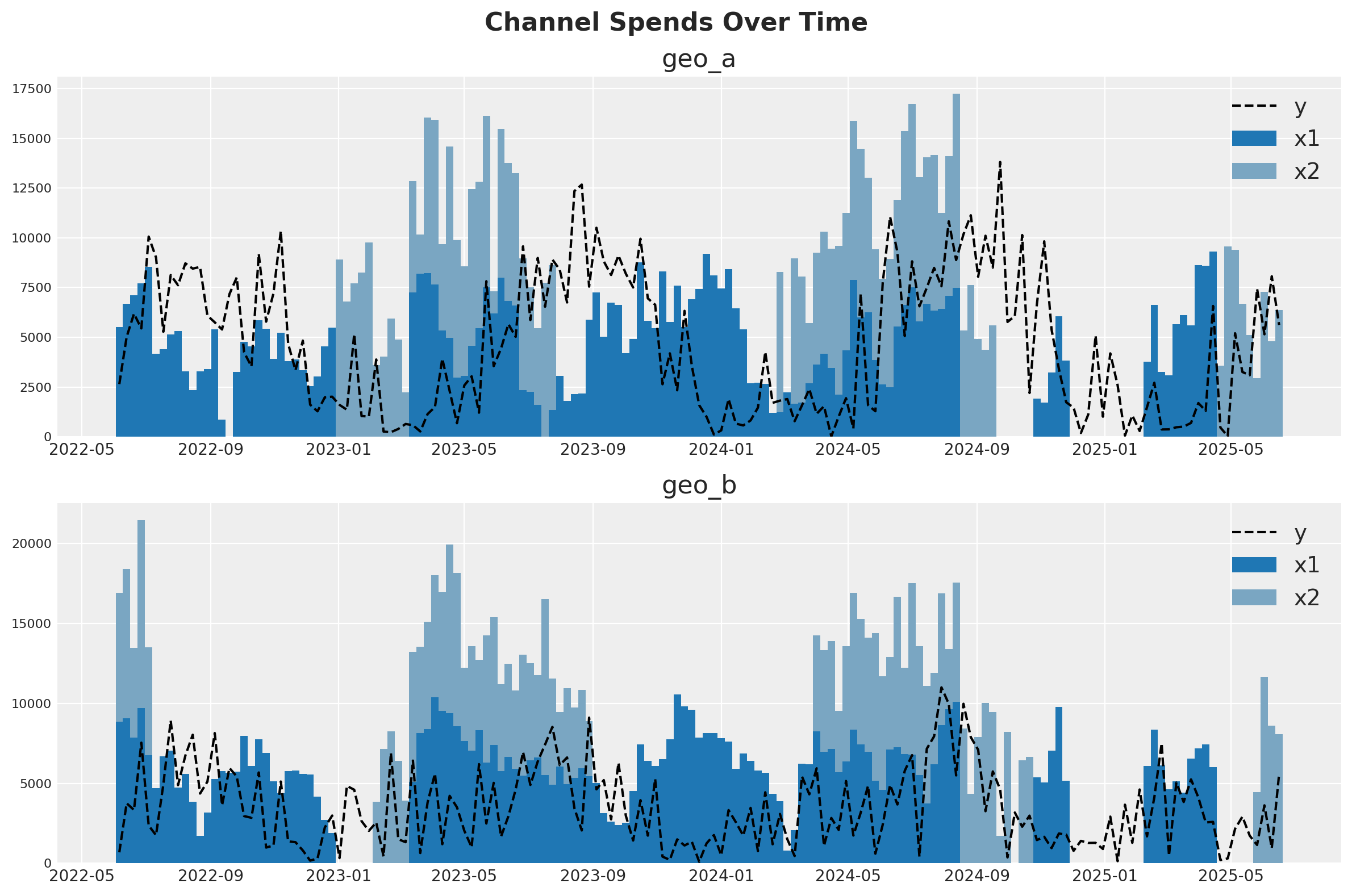
Para nuestro planteamiento, imagine que vendemos un producto en dos países distintos (geo_a y geo_b). Nuestro equipo de marketing gestiona dos canales: uno suele estar siempre activo y el otro es más táctico y se activa durante las campañas de marketing. La inspección visual de los datos sugiere que existe al menos algún efecto del marketing sobre las ventas, pero la relación es ruidosa. Nuestra misión es ver si el MMM puede separar la señal del ruido.
Una estrategia para tratar con datos ruidosos y de baja señal es aprovechar información de contextos similares. Si el canal 2 parece ser bastante efectivo en geo_b, eso nos da razones para sospechar que también lo será en geo_a. Esto puede implementarse con full pooling o partial pooling (los modelos de partial pooling a menudo se llaman “jerárquicos” o “multinivel”). Este cuaderno mostrará cómo ajustar un MMM a múltiples mercados al mismo tiempo y tomar decisiones sobre cómo agrupar información entre los dos contextos.
fig, (ax1, ax2) = plt.subplots(2, 1, figsize=(12, 8))
fig.suptitle("Channel Spends Over Time", fontsize=16, fontweight="bold")

blue_colors = ["#1f77b4", "#7aa6c2"]  # Darker and lighter shades of blue

# Plot for geo_a
geo_a_data = data_df[data_df["geo"] == "geo_a"]
ax1.bar(geo_a_data["date"], geo_a_data["x1"], label="x1", width=7, color=blue_colors[0])
ax1.bar(
    geo_a_data["date"],
    geo_a_data["x2"],
    bottom=geo_a_data["x1"],
    label="x2",
    width=7,
    color=blue_colors[1],
)
ax1.plot(geo_a_data["date"], geo_a_data["y"], "--", label="y", color="black")
ax1.set_title("geo_a")
ax1.legend()

# Plot for geo_b
geo_b_data = data_df[data_df["geo"] == "geo_b"]
ax2.bar(geo_b_data["date"], geo_b_data["x1"], label="x1", width=7, color=blue_colors[0])
ax2.bar(
    geo_b_data["date"],
    geo_b_data["x2"],
    bottom=geo_b_data["x1"],
    label="x2",
    width=7,
    color=blue_colors[1],
)
ax2.plot(geo_b_data["date"], geo_b_data["y"], "--", label="y", color="black")
ax2.set_title("geo_b")
ax2.legend()

plt.tight_layout()
Especificación de priors#
A product may perform very differently in distinct markets, popular in some locations but rather niche in others. If this is the case, observing how a product is doing in one market doesn’t tell us much about how it will be doing in another.
Alternatively, a product may behave very consistently across markets, either always loved or ignored. If so, we can better predict response across markets, including for those that we may only have noisy measurements.
More realistically, hierarchical models allow for a continuous interpolation between these two scenarios, adaptively pooling information to the extent it seems warranted. This is also called partial pooling. If you need an introduction on Bayesian hierarchical models, check out the comprehensive example «A Primer on Bayesian Methods for Multilevel Modeling» in the PyMC documentation.
This notebook we’ll illustrate hierarchical modeling in MMM models. This can be controlled via the dims argument of Prior objects used in model_config. We’ll show you how to code each type of assumption you might make (we aren’t recommending it as a good model!).
Let’s start with the beta parameter of the saturation curve, which represents the maximum number of weekly sales you could drive through a channel. It will be the only parameter we model hierarchically.
The beta_prior below has dimensions of channel and geo, meaning we will have one beta parameter per channel and per geographic market. The parameters, mu and std, also have a prior. But critically, they only have channel dimensions.
This forces the prior parameters to be shared across distinct geographies and, therefore, be compatible with all of them.
Specifically, the prior on mean captures what we expect each channel to do on average, without considering their variation on geography, while the prior on std represents how much the effect varies across geographies. std encodes the strength of «pooling». If it’s large, channels are expected to vary widely, if it’s small they are expected to be similarly behaved.
Note that distinct channels are still independent. If we wanted, we could have pooled information across channels by using a single mean and std prior shared between all channels and geographies.
beta_prior = LogNormalPrior(
    mean=Prior("Gamma", mu=0.25, sigma=0.10, dims="channel"),
    std=Prior("Exponential", scale=0.10, dims="channel"),
    dims=("channel", "geo"),
    centered=False,
)
Next we look at lambda, which represents the efficiency of a channel. The higher the lambda, the faster sales respond to spending on that channel. We’ll have the lambda parameter be fully pooled across all geographies. We are assuming that channel 1 has the same efficiency in both geographical markets, so we do not specify «geo» dims.
Note that by using constants for the parameters, there’s no shared learnable priors (i.e., hierarchical structure). This is what enforces a complete pooling structure.
lam_prior = Prior("Gamma", mu=0.5, sigma=0.25, dims="channel")

saturation = LogisticSaturation(
    priors={
        "beta": beta_prior,
        "lam": lam_prior,
    },
)
saturation.model_config
{'saturation_lam': Prior("Gamma", mu=0.5, sigma=0.25, dims="channel"),
 'saturation_beta': <pymc_marketing.special_priors.LogNormalPrior at 0x301c99e80>}
The alpha parameter of the Adstock function represents how long customers remember marketing. We’ll choose an unpooled structure. Here, each channel in each geography has its own effect and those effects do not influence each other. Notice that we put a dim for both geos and channels to indicate that we want 4 unique effects.
Once again we have no learnable parameters inside the prior of alpha. We could have tried to specify priors with the same dimensions geo and channel, which would still imply no-pooling of information. But if we did that, the model would become too undetermined, with each parameter prior only informed by one single alpha parameter each.
alpha_prior = Prior("Beta", alpha=2, beta=5, dims=("geo", "channel"))

adstock = GeometricAdstock(
    priors={"alpha": alpha_prior},
    l_max=8,
)

adstock.model_config
{'adstock_alpha': Prior("Beta", alpha=2, beta=5, dims=("geo", "channel"))}
You can mix and match the unpooled, fully pooled, and partially pooled strategy for any of your effects. You can extend this strategy to controls or noise parameters as well. Given the variety of options, it can be hard to know which pooling strategy to choose for a given effect. In our opinion, the choice is primarily driven by computational considerations. Partial pooling is generally a more reasonable assumption, but it can make the model slower or harder to estimate, and more difficult to reason about.
For example, you might notice that we set our beta prior with centered=False. This is known as a reparameterization, a strategy to solve computational difficulties that MCMC algorithms can run into when fitting hierarchical models, specially with small dimensions (remember we have just two channels and two geographies!).
We recommend that you start with a model that uses only fully pooled or unpooled effects. Once you have a good working model you can add complexity slowly, verifying your model performance and accuracy at each stage.
Completamos la especificación del modelo con priors similares a los de Cuaderno de ejemplo para MMM.
model_config = {
    "intercept": Prior("Gamma", mu=0.5, sigma=0.25, dims="geo"),
    "gamma_control": Prior("Normal", mu=0, sigma=0.5, dims="control"),
    "gamma_fourier": LaplacePrior(
        mu=0,
        b=Prior("HalfNormal", sigma=0.2),
        dims=("geo", "fourier_mode"),
        centered=False,
    ),
    "likelihood": Prior(
        "TruncatedNormal",
        lower=0,
        sigma=Prior("HalfNormal", sigma=1.5),
        dims=("date", "geo"),
    ),
}
Definición del modelo#
Ya estamos listos para definir la clase del modelo. La API es muy similar a la de Cuaderno de ejemplo para MMM.
# Base MMM model specification
mmm = MMM(
    date_column="date",
    target_column="y",
    channel_columns=["x1", "x2"],
    control_columns=["event_1", "event_2"],
    dims=("geo",),
    scaling={
        "channel": {"method": "max", "dims": ()},
        "target": {"method": "max", "dims": ()},
    },
    adstock=adstock,
    saturation=saturation,
    yearly_seasonality=2,
    model_config=model_config,
)
Truco
Observa que tenemos los dos argumentos nuevos siguientes:
dims: una tupla de cadenas de texto que especifica las dimensiones del modelo.scaling: un diccionario que especifica el método de escalado y las dimensiones para la variable objetivo y las variables de medios. En este caso dejamos las dimensiones vacías porque queremos escalar la variable objetivo por cada geo (ver detalles abajo).
Ahora podemos preparar los datos de entrenamiento.
x_train = data_df.drop(columns=["y"])
y_train = data_df["y"]
Para construir el modelo, necesitamos especificar los datos de entrenamiento y las variables objetivo.
Truco
No necesitamos construir el modelo; simplemente podemos ajustarlo. Esto es solo para inspeccionar la estructura del modelo.
mmm.build_model(X=x_train, y=y_train)
Veamos el grafo del modelo:
mmm.model.to_graphviz()

It may be easier to visualize the dimensions of each parameter in a table format:
mmm.table()
                             Variable  Expression                             Dimensions
───────────────────────────────────────────────────────────────────────────────────────────────────────────────────
                      channel_scale =  Data                                   geo[2] × channel[2]
                       target_scale =  Data                                   geo[2]
                       channel_data =  Data                                   date[159] × geo[2] × channel[2]
                        target_data =  Data                                   date[159] × geo[2]
                       control_data =  Data                                   date[159] × geo[2] × control[2]
                          dayofyear =  Data                                   date[159]

             intercept_contribution ~  Gamma(f(), f())                        geo[2]
                      adstock_alpha ~  Beta(2, 5)                             geo[2] × channel[2]
                     saturation_lam ~  Gamma(f(), f())                        channel[2]
               saturation_beta_mean ~  Gamma(f(), f())                        channel[2]
                saturation_beta_std ~  Exponential(0.1)                       channel[2]
         saturation_beta_log_offset ~  Normal(0, 1)                           channel[2] × geo[2]
                      gamma_control ~  Normal(0, 0.5)                         control[2]
                    gamma_fourier_b ~  HalfNormal(0, 0.2)
                gamma_fourier_sigma ~  Exponential(f(gamma_fourier_b))
               gamma_fourier_offset ~  Normal(0, 1)                           geo[2] × fourier_mode[4]
                            y_sigma ~  HalfNormal(0, 1.5)
                                                                              Parameter count = 29

                    saturation_beta =  f(saturation_beta_log_offset,          channel[2] × geo[2]
                                       saturation_beta_mean,
                                       saturation_beta_std)
               channel_contribution =  f(saturation_lam,                      date[159] × geo[2] × channel[2]
                                       saturation_beta_log_offset,
                                       saturation_beta_mean, adstock_alpha,
                                       saturation_beta_std)
 total_media_contribution_original_s…  f(saturation_lam,
                                    =  saturation_beta_log_offset,
                                       saturation_beta_mean, adstock_alpha,
                                       saturation_beta_std)
               control_contribution =  f(gamma_control)                       date[159] × geo[2] × control[2]
                      gamma_fourier =  f(gamma_fourier_offset,                geo[2] × fourier_mode[4]
                                       gamma_fourier_sigma)
               fourier_contribution =  f(gamma_fourier_offset,                date[159] × geo[2] × fourier_mode[4]
                                       gamma_fourier_sigma)
    yearly_seasonality_contribution =  f(gamma_fourier_offset,                date[159] × geo[2]
                                       gamma_fourier_sigma)

                                  y ~  TruncatedNormal(f(intercept_contribu…  date[159] × geo[2]
                                       gamma_control, gamma_fourier_offset,
                                       gamma_fourier_sigma, saturation_lam,
                                       saturation_beta_log_offset,
                                       saturation_beta_mean, adstock_alpha,
                                       saturation_beta_std), y_sigma, 0,
                                       inf)
¡Es genial ver que el modelo se vectoriza automáticamente y crea las jerarquías y dimensiones esperadas 🚀!
Como estamos escalando nuestros datos internamente, podemos añadir términos deterministas para recuperar las contribuciones de los componentes en la escala original.
mmm.add_original_scale_contribution_variable(
    var=[
        "channel_contribution",
        "control_contribution",
        "intercept_contribution",
        "yearly_seasonality_contribution",
        "y",
    ]
)

pm.model_to_graphviz(mmm.model)

Volviendo a los escaladores, podemos obtenerlos como un dataset de xarray.
scalers = mmm.get_scales_as_xarray()

scalers
{'channel_scale': <xarray.DataArray '_channel' (geo: 2, channel: 2)> Size: 32B
 array([[ 9318.97848455,  9755.9729876 ],
        [10555.0774866 , 11760.98180037]])
 Coordinates:
   * geo      (geo) object 16B 'geo_a' 'geo_b'
   * channel  (channel) object 16B 'x1' 'x2',
 'target_scale': <xarray.DataArray '_target' (geo: 2)> Size: 16B
 array([13812.08025674, 11002.97913936])
 Coordinates:
   * geo      (geo) object 16B 'geo_a' 'geo_b'}
Como era de esperar por la definición del modelo, tenemos escaladores para la variable objetivo y las variables de medios en todas las geos.
Comprobaciones predictivas previas#
Antes de ajustar el modelo, podemos inspeccionar la distribución predictiva previa.
with mmm.model:
    prior = pm.sample_prior_predictive()
prior
Sampling: [adstock_alpha, gamma_control, gamma_fourier_b, gamma_fourier_offset, gamma_fourier_sigma, intercept_contribution, saturation_beta_log_offset, saturation_beta_mean, saturation_beta_std, saturation_lam, y, y_sigma]
-
<xarray.Dataset> Size: 19MB Dimensions: (chain: 1, draw: 500, geo: 2, channel: 2, date: 159, control: 2, fourier_mode: 4) Coordinates: * chain (chain) int64 8B 0 * draw (draw) int64 4kB 0 1 ... 499 * geo (geo) <U5 40B 'geo_a' 'ge... * channel (channel) <U2 16B 'x1' 'x2' * date (date) datetime64[ns] 1kB ... * control (control) <U7 56B 'event_... * fourier_mode (fourier_mode) <U5 80B 's... Data variables: (12/23) adstock_alpha (chain, draw, geo, channel) float64 16kB ... channel_contribution (chain, draw, date, geo, channel) float64 3MB ... channel_contribution_original_scale (chain, draw, date, geo, channel) float64 3MB ... control_contribution (chain, draw, date, geo, control) float64 3MB ... control_contribution_original_scale (chain, draw, date, geo, control) float64 3MB ... fourier_contribution (chain, draw, date, geo, fourier_mode) float64 5MB ... ... ... saturation_lam (chain, draw, channel) float64 8kB ... total_media_contribution_original_scale (chain, draw) float64 4kB ... y_original_scale (chain, draw, date, geo) float64 1MB ... y_sigma (chain, draw) float64 4kB ... yearly_seasonality_contribution (chain, draw, date, geo) float64 1MB ... yearly_seasonality_contribution_original_scale (chain, draw, date, geo) float64 1MB ... Attributes: created_at: 2026-01-26T15:51:06.153383+00:00 arviz_version: 0.23.0 inference_library: pymc inference_library_version: 5.27.0 -
<xarray.Dataset> Size: 1MB Dimensions: (chain: 1, draw: 500, date: 159, geo: 2) Coordinates: * chain (chain) int64 8B 0 * draw (draw) int64 4kB 0 1 2 3 4 5 6 7 ... 493 494 495 496 497 498 499 * date (date) datetime64[ns] 1kB 2022-06-06 2022-06-13 ... 2025-06-16 * geo (geo) <U5 40B 'geo_a' 'geo_b' Data variables: y (chain, draw, date, geo) float64 1MB 0.3768 1.362 ... 0.51 0.298 Attributes: created_at: 2026-01-26T15:51:06.158696+00:00 arviz_version: 0.23.0 inference_library: pymc inference_library_version: 5.27.0 -
<xarray.Dataset> Size: 4kB Dimensions: (date: 159, geo: 2) Coordinates: * date (date) datetime64[ns] 1kB 2022-06-06 2022-06-13 ... 2025-06-16 * geo (geo) <U5 40B 'geo_a' 'geo_b' Data variables: y (date, geo) float64 3kB 0.1917 0.06202 0.3635 ... 0.4068 0.5073 Attributes: created_at: 2026-01-26T15:51:06.159453+00:00 arviz_version: 0.23.0 inference_library: pymc inference_library_version: 5.27.0 -
<xarray.Dataset> Size: 12kB
Dimensions:        (date: 159, geo: 2, channel: 2, control: 2)
Coordinates:
  * date           (date) datetime64[ns] 1kB 2022-06-06 ... 2025-06-16
  * geo            (geo) <U5 40B 'geo_a' 'geo_b'
  * channel        (channel) <U2 16B 'x1' 'x2'
  * control        (control) <U7 56B 'event_1' 'event_2'
Data variables:
    channel_data   (date, geo, channel) float64 5kB 5.528e+03 0.0 ... 8.091e+03
    channel_scale  (geo, channel) float64 32B 9.319e+03 9.756e+03 ... 1.176e+04
    control_data   (date, geo, control) int32 3kB 0 0 0 0 0 0 0 ... 0 0 0 0 0 0
    dayofyear      (date) int32 636B 157 164 171 178 185 ... 139 146 153 160 167
    target_data    (date, geo) float64 3kB 2.648e+03 682.4 ... 5.581e+03
    target_scale   (geo) float64 16B 1.381e+04 1.1e+04
Attributes:
    created_at:                 2026-01-26T15:51:06.161746+00:00
    arviz_version:              0.23.0
    inference_library:          pymc
    inference_library_version:  5.27.0
g = sns.relplot(
    data=data_df,
    x="date",
    y="y",
    color="black",
    col="geo",
    col_wrap=1,
    kind="line",
    height=4,
    aspect=3,
)

axes = g.axes.flatten()

for ax, geo in zip(axes, mmm.model.coords["geo"], strict=True):
    az.plot_hdi(
        x=mmm.model.coords["date"],
        y=(
            prior.prior.sel(geo=geo)["y_original_scale"]
            .unstack()
            .transpose(..., "date")
        ),
        smooth=False,
        color="C0",
        hdi_prob=0.94,
        fill_kwargs={"alpha": 0.3, "label": "94% HDI"},
        ax=ax,
    )
    az.plot_hdi(
        x=mmm.model.coords["date"],
        y=(
            prior.prior.sel(geo=geo)["y_original_scale"]
            .unstack()
            .transpose(..., "date")
        ),
        smooth=False,
        color="C0",
        hdi_prob=0.5,
        fill_kwargs={"alpha": 0.5, "label": "50% HDI"},
        ax=ax,
    )
    ax.legend(loc="upper left")

g.figure.suptitle("Prior Predictive", fontsize=16, fontweight="bold", y=1.03);
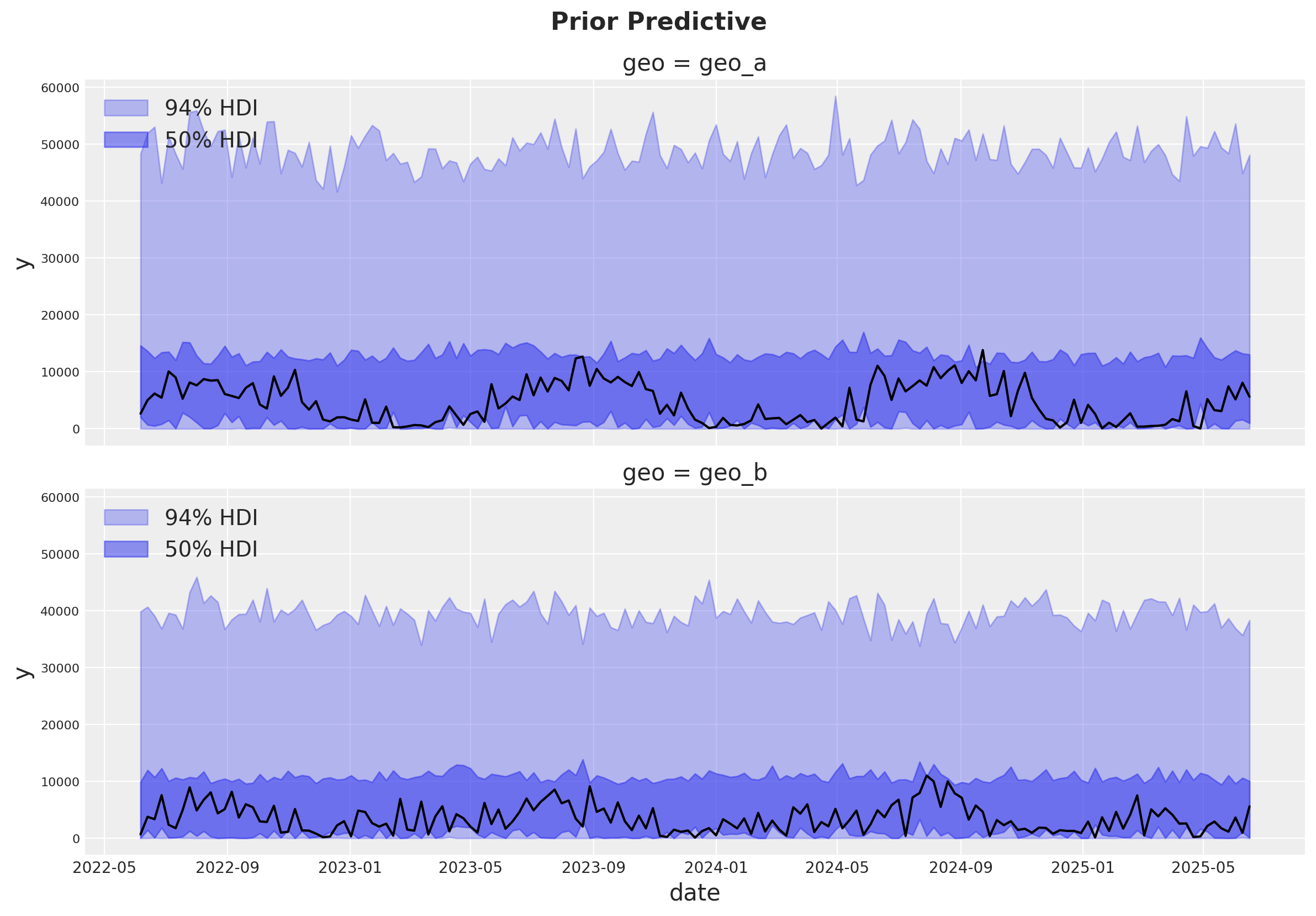
La distribución predictiva previa se ve bien y no es demasiado restrictiva.
Ajuste del modelo#
Ahora podemos ajustar el modelo y generar la distribución predictiva posterior.
mmm.fit(
    X=x_train,
    y=y_train,
    chains=4,
    target_accept=0.95,
    random_seed=rng,
)

mmm.sample_posterior_predictive(
    X=x_train,
    random_seed=rng,
)
Initializing NUTS using jitter+adapt_diag...
Multiprocess sampling (4 chains in 4 jobs)
NUTS: [intercept_contribution, adstock_alpha, saturation_lam, saturation_beta_mean, saturation_beta_std, saturation_beta_log_offset, gamma_control, gamma_fourier_b, gamma_fourier_sigma, gamma_fourier_offset, y_sigma]
Sampling 4 chains for 1_000 tune and 1_000 draw iterations (4_000 + 4_000 draws total) took 11 seconds.
Sampling: [y]
<xarray.Dataset> Size: 20MB
Dimensions:           (date: 159, geo: 2, sample: 4000)
Coordinates:
  * date              (date) datetime64[ns] 1kB 2022-06-06 ... 2025-06-16
  * geo               (geo) <U5 40B 'geo_a' 'geo_b'
  * sample            (sample) object 32kB MultiIndex
  * chain             (sample) int64 32kB 0 0 0 0 0 0 0 0 0 ... 3 3 3 3 3 3 3 3
  * draw              (sample) int64 32kB 0 1 2 3 4 5 ... 995 996 997 998 999
Data variables:
    y                 (date, geo, sample) float64 10MB 0.5281 0.6166 ... 0.04538
    y_original_scale  (date, geo, sample) float64 10MB 7.295e+03 ... 499.3
Attributes:
    created_at:                 2026-01-26T15:51:22.357324+00:00
    arviz_version:              0.23.0
    inference_library:          pymc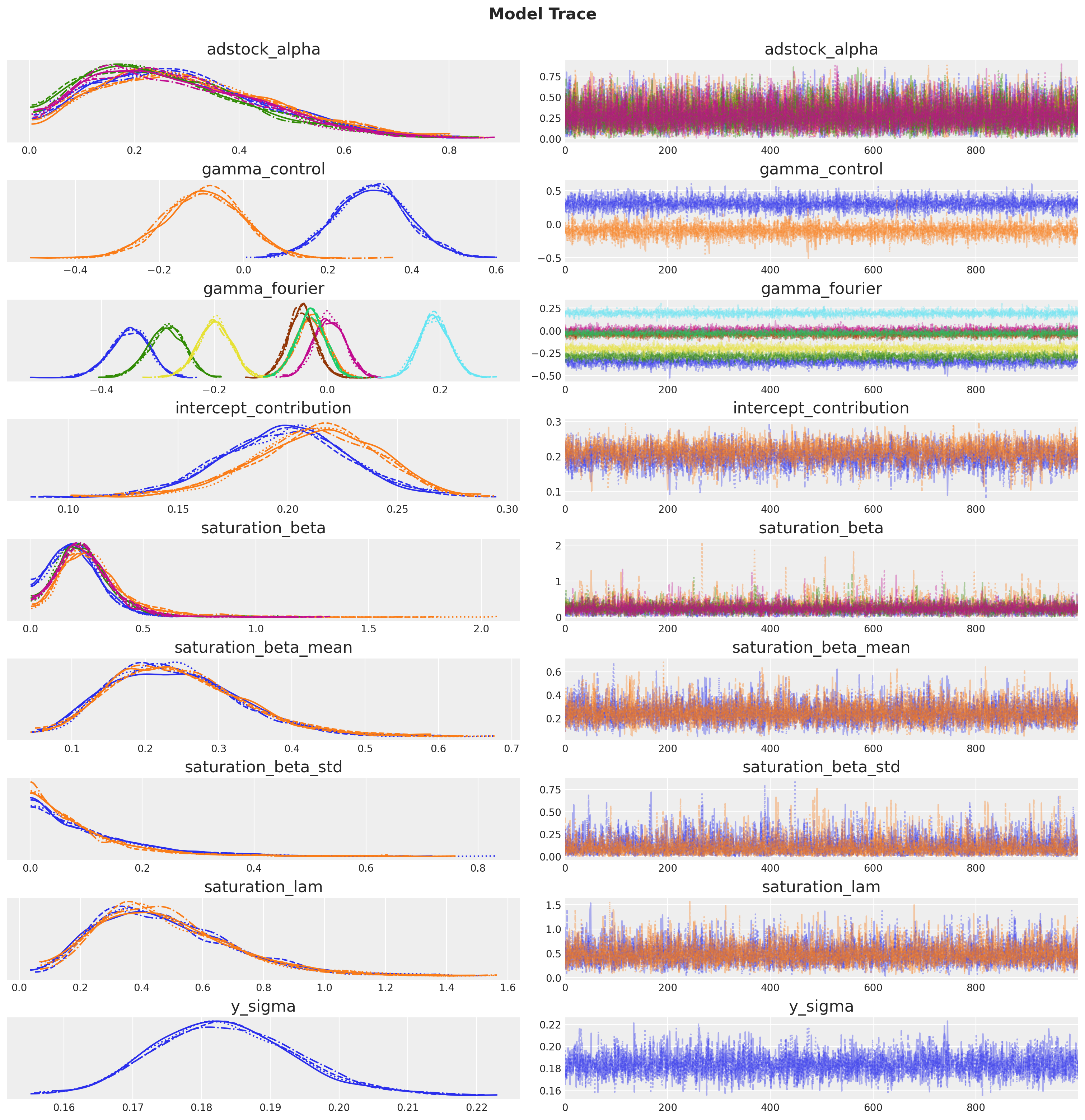
inference_library_version: 5.27.0El muestreo se ve bien. No hay divergencias y los valores de r-hat están cercanos a \(1\).
mmm.idata.sample_stats.diverging.sum("draw")
<xarray.DataArray 'diverging' (chain: 4)> Size: 32B
array([0, 0, 0, 0])
Coordinates:
  * chain    (chain) int64 32B 0 1 2 3
az.summary(
    mmm.idata,
    var_names=[
        "adstock_alpha",
        "gamma_control",
        "gamma_fourier",
        "intercept_contribution",
        "saturation_beta",
        "saturation_beta_mean",
        "saturation_beta_std",
        "saturation_lam",
        "y_sigma",
    ],
)
| mean | sd | hdi_3% | hdi_97% | mcse_mean | mcse_sd | ess_bulk | ess_tail | r_hat | |
|---|---|---|---|---|---|---|---|---|---|
| adstock_alpha[geo_a, x1] | 0.294 | 0.160 | 0.028 | 0.587 | 0.002 | 0.002 | 5818.0 | 2660.0 | 1.0 |
| adstock_alpha[geo_a, x2] | 0.306 | 0.165 | 0.038 | 0.614 | 0.002 | 0.003 | 6170.0 | 2233.0 | 1.0 |
| adstock_alpha[geo_b, x1] | 0.262 | 0.155 | 0.021 | 0.554 | 0.002 | 0.003 | 5405.0 | 2760.0 | 1.0 |
| adstock_alpha[geo_b, x2] | 0.278 | 0.157 | 0.023 | 0.555 | 0.002 | 0.003 | 6615.0 | 2591.0 | 1.0 |
| gamma_control[event_1] | 0.304 | 0.086 | 0.152 | 0.479 | 0.001 | 0.001 | 4907.0 | 2767.0 | 1.0 |
| gamma_control[event_2] | -0.096 | 0.092 | -0.267 | 0.075 | 0.001 | 0.002 | 5247.0 | 3088.0 | 1.0 |
| gamma_fourier[geo_a, sin_1] | -0.350 | 0.035 | -0.419 | -0.290 | 0.001 | 0.000 | 3874.0 | 3353.0 | 1.0 |
| gamma_fourier[geo_a, sin_2] | -0.029 | 0.028 | -0.080 | 0.023 | 0.000 | 0.000 | 5379.0 | 3577.0 | 1.0 |
| gamma_fourier[geo_a, cos_1] | -0.285 | 0.033 | -0.350 | -0.228 | 0.001 | 0.000 | 3965.0 | 4005.0 | 1.0 |
| gamma_fourier[geo_a, cos_2] | 0.004 | 0.028 | -0.049 | 0.055 | 0.000 | 0.000 | 5619.0 | 3294.0 | 1.0 |
| gamma_fourier[geo_b, sin_1] | -0.046 | 0.025 | -0.094 | 0.001 | 0.000 | 0.000 | 6727.0 | 3069.0 | 1.0 |
| gamma_fourier[geo_b, sin_2] | 0.191 | 0.027 | 0.137 | 0.240 | 0.000 | 0.000 | 5103.0 | 2933.0 | 1.0 |
| gamma_fourier[geo_b, cos_1] | -0.200 | 0.030 | -0.259 | -0.146 | 0.000 | 0.000 | 4215.0 | 3060.0 | 1.0 |
| gamma_fourier[geo_b, cos_2] | -0.030 | 0.026 | -0.079 | 0.017 | 0.000 | 0.000 | 6318.0 | 3127.0 | 1.0 |
| intercept_contribution[geo_a] | 0.199 | 0.028 | 0.147 | 0.254 | 0.000 | 0.000 | 3372.0 | 2642.0 | 1.0 |
| intercept_contribution[geo_b] | 0.212 | 0.029 | 0.158 | 0.265 | 0.001 | 0.001 | 2497.0 | 1769.0 | 1.0 |
| saturation_beta[x1, geo_a] | 0.199 | 0.111 | 0.004 | 0.387 | 0.002 | 0.002 | 4504.0 | 3296.0 | 1.0 |
| saturation_beta[x1, geo_b] | 0.284 | 0.171 | 0.007 | 0.563 | 0.003 | 0.006 | 2969.0 | 2716.0 | 1.0 |
| saturation_beta[x2, geo_a] | 0.236 | 0.128 | 0.004 | 0.443 | 0.002 | 0.003 | 5570.0 | 2888.0 | 1.0 |
| saturation_beta[x2, geo_b] | 0.242 | 0.133 | 0.013 | 0.463 | 0.002 | 0.003 | 4851.0 | 2987.0 | 1.0 |
| saturation_beta_mean[x1] | 0.241 | 0.088 | 0.090 | 0.404 | 0.001 | 0.002 | 5311.0 | 2763.0 | 1.0 |
| saturation_beta_mean[x2] | 0.245 | 0.091 | 0.082 | 0.412 | 0.001 | 0.002 | 5807.0 | 2482.0 | 1.0 |
| saturation_beta_std[x1] | 0.111 | 0.105 | 0.000 | 0.305 | 0.002 | 0.002 | 3322.0 | 2208.0 | 1.0 |
| saturation_beta_std[x2] | 0.093 | 0.096 | 0.000 | 0.261 | 0.001 | 0.002 | 4072.0 | 1918.0 | 1.0 |
| saturation_lam[x1] | 0.475 | 0.221 | 0.118 | 0.882 | 0.003 | 0.004 | 4577.0 | 2354.0 | 1.0 |
| saturation_lam[x2] | 0.477 | 0.218 | 0.128 | 0.890 | 0.003 | 0.004 | 6169.0 | 3033.0 | 1.0 |
| y_sigma | 0.183 | 0.010 | 0.166 | 0.204 | 0.000 | 0.000 | 3781.0 | 3144.0 | 1.0 |
_ = az.plot_trace(
    data=mmm.idata,
    var_names=[
        "adstock_alpha",
        "gamma_control",
        "gamma_fourier",
        "intercept_contribution",
        "saturation_beta",
        "saturation_beta_mean",
        "saturation_beta_std",
        "saturation_lam",
        "y_sigma",
    ],
    compact=True,
    backend_kwargs={"figsize": (15, 15), "layout": "constrained"},
)
plt.gcf().suptitle("Model Trace", fontsize=16, fontweight="bold", y=1.03);
Comprobaciones predictivas posteriores#
Ahora podemos inspeccionar la distribución predictiva posterior. Como antes, necesitamos escalar la predictiva posterior a la escala original para hacerla comparable con los datos.
fig, axes = plt.subplots(
    nrows=len(mmm.model.coords["geo"]),
    figsize=(12, 9),
    sharex=True,
    sharey=True,
    layout="constrained",
)

for i, geo in enumerate(mmm.model.coords["geo"]):
    ax = axes[i]
    az.plot_hdi(
        x=mmm.model.coords["date"],
        y=(mmm.idata["posterior_predictive"].y_original_scale.sel(geo=geo)),
        color="C0",
        smooth=False,
        hdi_prob=0.94,
        fill_kwargs={"alpha": 0.2, "label": "94% HDI"},
        ax=ax,
    )

    az.plot_hdi(
        x=mmm.model.coords["date"],
        y=(mmm.idata["posterior_predictive"].y_original_scale.sel(geo=geo)),
        color="C0",
        smooth=False,
        hdi_prob=0.5,
        fill_kwargs={"alpha": 0.4, "label": "50% HDI"},
        ax=ax,
    )

    sns.lineplot(
        data=data_df.query("geo == @geo"),
        x="date",
        y="y",
        color="black",
        ax=ax,
    )

    ax.legend(loc="upper left")
    ax.set(title=f"{geo}")

fig.suptitle("Posterior Predictive", fontsize=16, fontweight="bold", y=1.03);
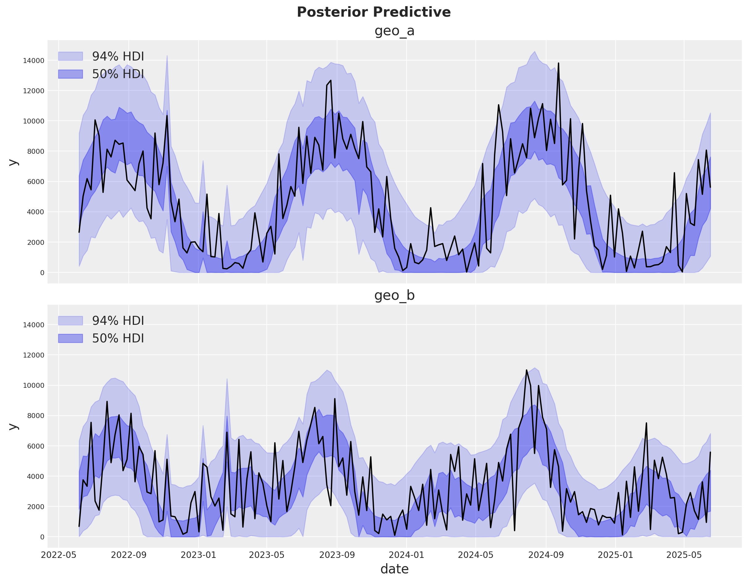
¡El ajuste se ve bien! Hay mucho ruido blanco en el proceso de ventas que no podemos predecir. Sin embargo, los movimientos principales en las ventas están capturados ya sea por nuestro modelo de estacionalidad o por los componentes del MMM.
Componentes del modelo#
Podemos extraer las contribuciones de cada componente del modelo en la escala original gracias a las variables deterministas añadidas al modelo.
fig, axes = plt.subplots(
    nrows=len(mmm.model.coords["geo"]),
    figsize=(15, 10),
    sharex=True,
    sharey=True,
    layout="constrained",
)

for i, geo in enumerate(mmm.model.coords["geo"]):
    ax = axes[i]

    for j, channel in enumerate(mmm.model.coords["channel"]):
        az.plot_hdi(
            x=mmm.model.coords["date"],
            y=mmm.idata["posterior"]["channel_contribution_original_scale"].sel(
                geo=geo, channel=channel
            ),
            color=f"C{j}",
            smooth=False,
            hdi_prob=0.94,
            fill_kwargs={"alpha": 0.5, "label": f"94% HDI ({channel})"},
            ax=ax,
        )

    az.plot_hdi(
        x=mmm.model.coords["date"],
        y=mmm.idata["posterior"]["intercept_contribution_original_scale"]
        .sel(geo=geo)
        .expand_dims({"date": mmm.model.coords["date"]})
        .transpose(..., "date"),
        color="C2",
        smooth=False,
        hdi_prob=0.94,
        fill_kwargs={"alpha": 0.5, "label": "94% HDI intercept"},
        ax=ax,
    )

    az.plot_hdi(
        x=mmm.model.coords["date"],
        y=mmm.idata["posterior"]["yearly_seasonality_contribution_original_scale"].sel(
            geo=geo,
        ),
        color="C3",
        smooth=False,
        hdi_prob=0.94,
        fill_kwargs={"alpha": 0.5, "label": "94% HDI Fourier"},
        ax=ax,
    )

    for k, control in enumerate(mmm.model.coords["control"]):
        az.plot_hdi(
            x=mmm.model.coords["date"],
            y=mmm.idata["posterior"]["control_contribution_original_scale"].sel(
                geo=geo, control=control
            ),
            color=f"C{5 + k}",
            smooth=False,
            hdi_prob=0.94,
            fill_kwargs={"alpha": 0.5, "label": f"94% HDI control ({control})"},
            ax=ax,
        )

    sns.lineplot(
        data=data_df.query("geo == @geo"),
        x="date",
        y="y",
        color="black",
        label="y",
        ax=ax,
    )
    ax.legend(
        loc="upper center",
        bbox_to_anchor=(0.5, -0.1),
        ncol=4,
    )
    ax.set(title=f"{geo}")

fig.suptitle(
    "Posterior Predictive - Channel Contributions",
    fontsize=16,
    fontweight="bold",
    y=1.03,
);
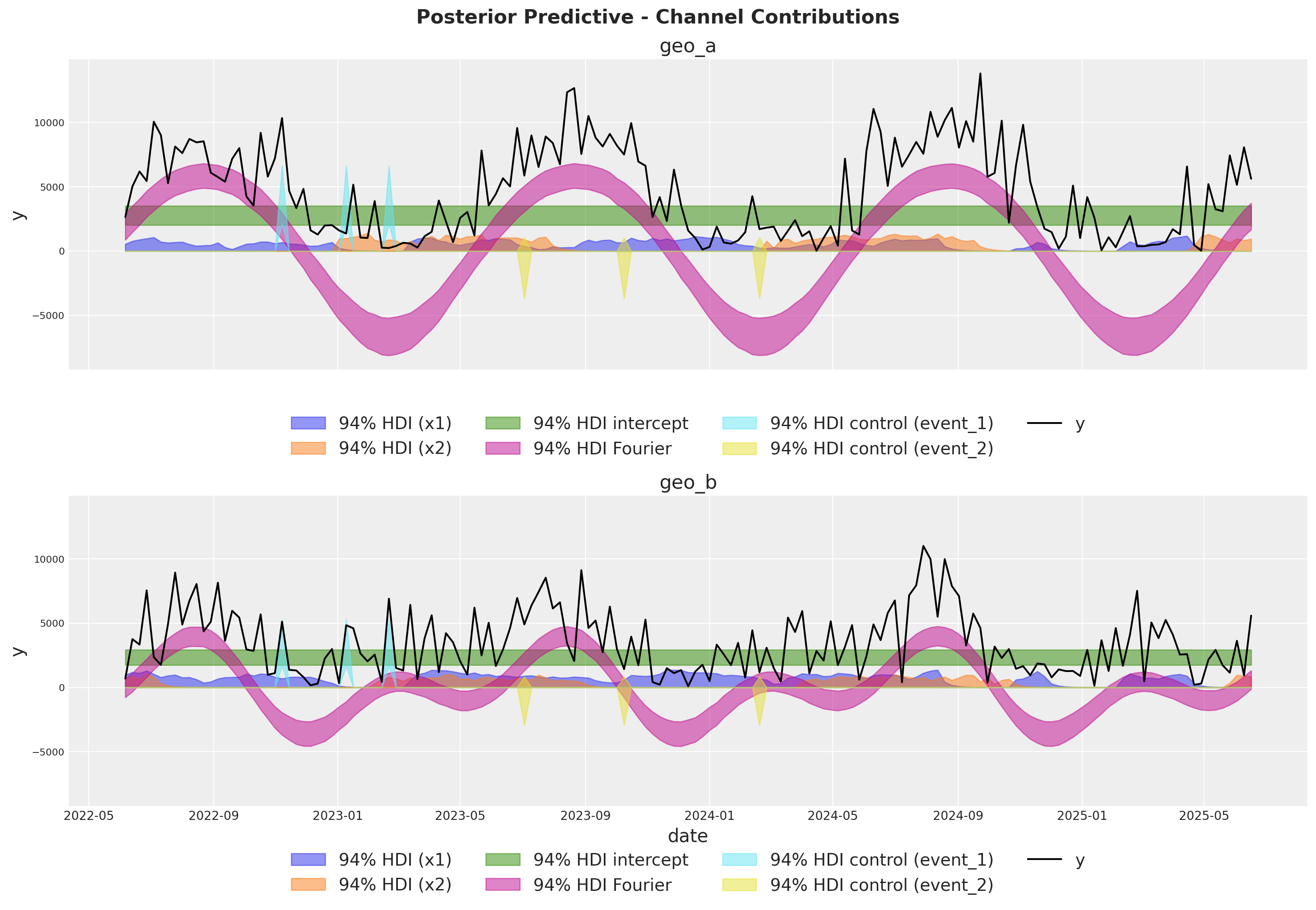
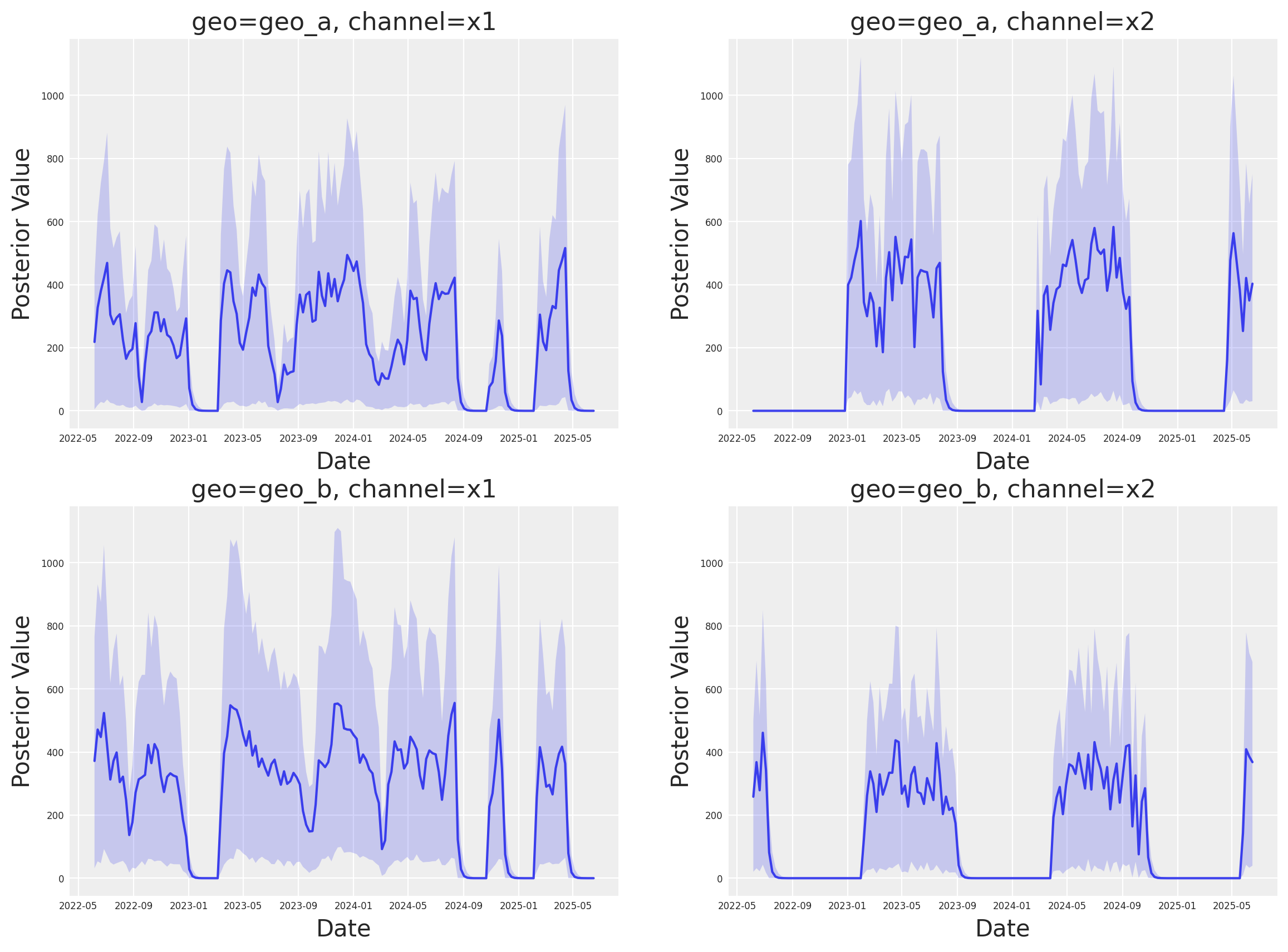
Análisis profundo de medios#
A continuación, podemos analizar las contribuciones individuales por canal en las distintas geos. Esta nueva clase tiene un nuevo espacio de nombres plot que contiene muchos métodos de visualización.
fig, axes = mmm.plot.contributions_over_time(
    var=["channel_contribution_original_scale"],
)

# Adjust figure size and layout to 2x2
fig.set_size_inches(14, 10)
fig.set_constrained_layout(True)

# Reshape axes to 2x2 grid
num_axes = len(axes.flatten())
if num_axes > 0:
    # Create a new 2x2 grid
    gs = fig.add_gridspec(2, 2)

    # Move existing axes to the new grid
    for i, ax in enumerate(axes.flatten()):
        if i < 4:  # Only handle up to 4 axes for 2x2 grid
            ax.set_position(gs[i // 2, i % 2].get_position(fig))

axes = axes.flatten()

# Share x and y axes across all subplots
for ax in axes:
    ax.legend().remove()
    ax.tick_params(axis="both", which="major", labelsize=6)
    ax.tick_params(axis="both", which="minor", labelsize=6)

# Share y axis limits
y_min = min(ax.get_ylim()[0] for ax in axes)
y_max = max(ax.get_ylim()[1] for ax in axes)
for ax in axes:
    ax.set_ylim(y_min, y_max)

# Share x axis limits
x_min = min(ax.get_xlim()[0] for ax in axes)
x_max = max(ax.get_xlim()[1] for ax in axes)
for ax in axes:
    ax.set_xlim(x_min, x_max)
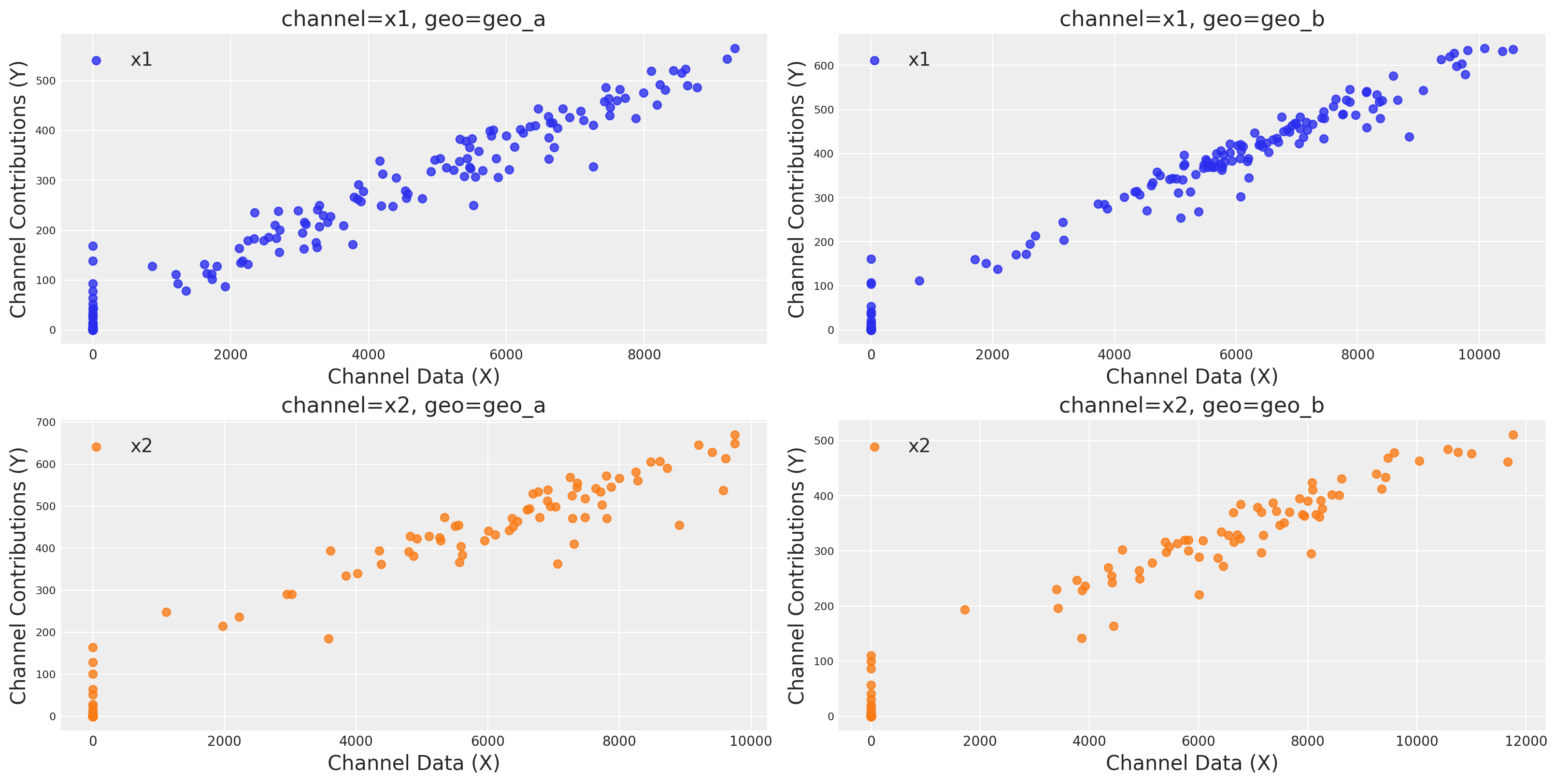
Podemos graficar las curvas de saturación para cada canal y geo usando varias funciones diferentes:
Usando
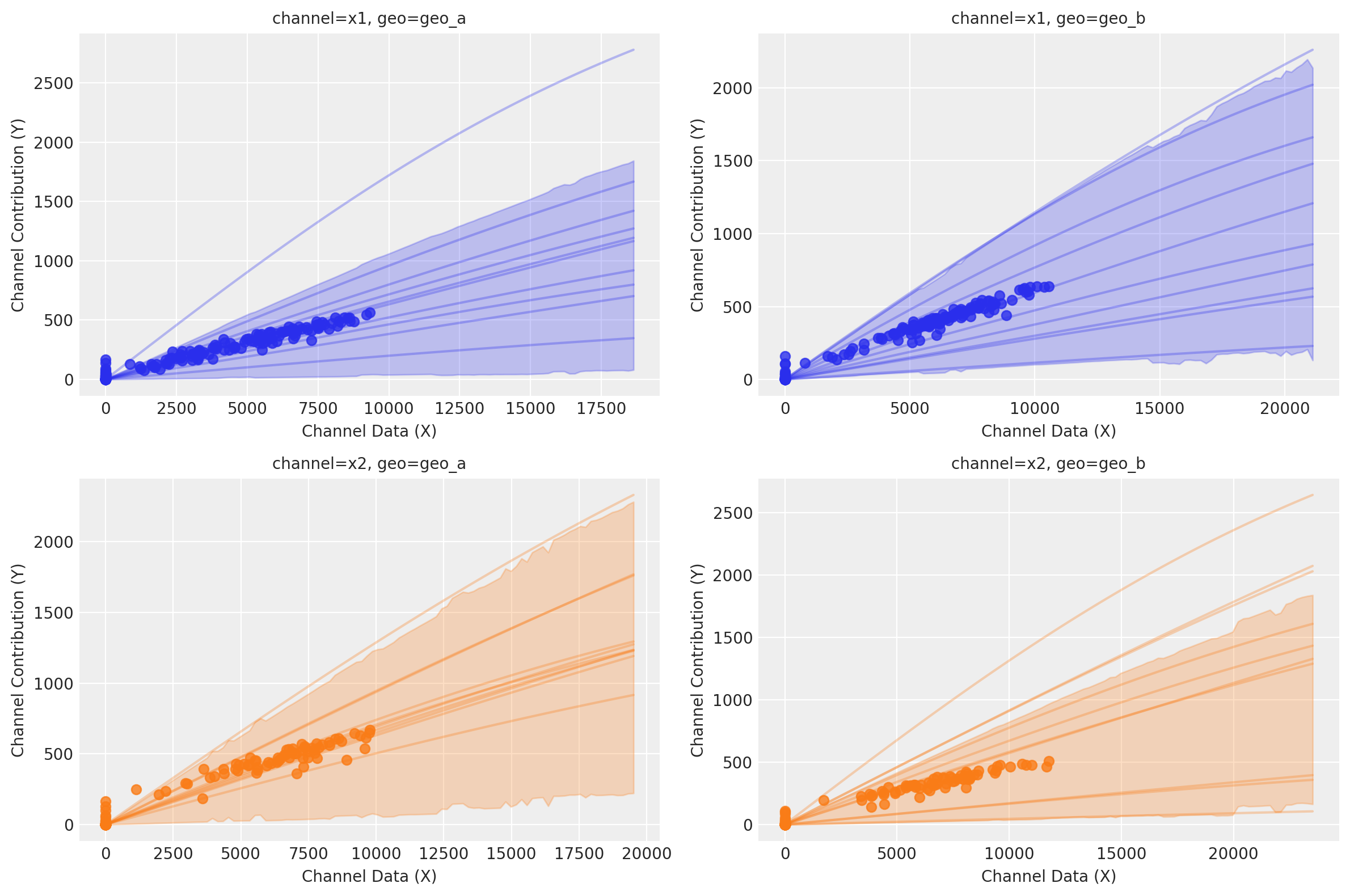
saturation_scatterplot, podemos obtener únicamente el diagrama de dispersión entre inversión y retornos estimados.Usando
saturation_curves, podemos obtener la posterior de las curvas y su ajuste posterior respecto a la contribución media dada.
mmm.plot.saturation_scatterplot(width_per_col=8, height_per_row=4, original_scale=True);
curve = mmm.saturation.sample_curve(mmm.idata.posterior, max_value=2)
fig, axes = mmm.plot.saturation_curves(
    curve,
    original_scale=True,
    n_samples=10,
    hdi_probs=0.85,
    random_seed=rng,
    subplot_kwargs={"figsize": (12, 8), "ncols": 2},
    rc_params={
        "xtick.labelsize": 10,
        "ytick.labelsize": 10,
        "axes.labelsize": 10,
        "axes.titlesize": 10,
    },
)

for ax in axes.ravel():
    ax.title.set_fontsize(10)

if fig._suptitle is not None:
    fig._suptitle.set_fontsize(12)

plt.tight_layout()
plt.show()
Sampling: []
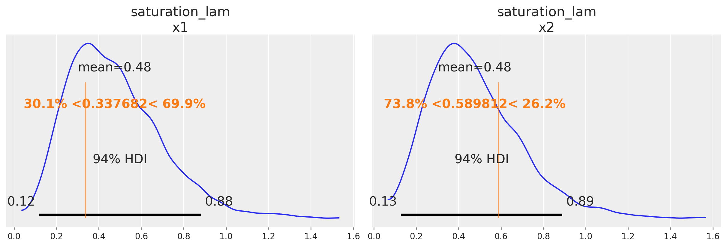
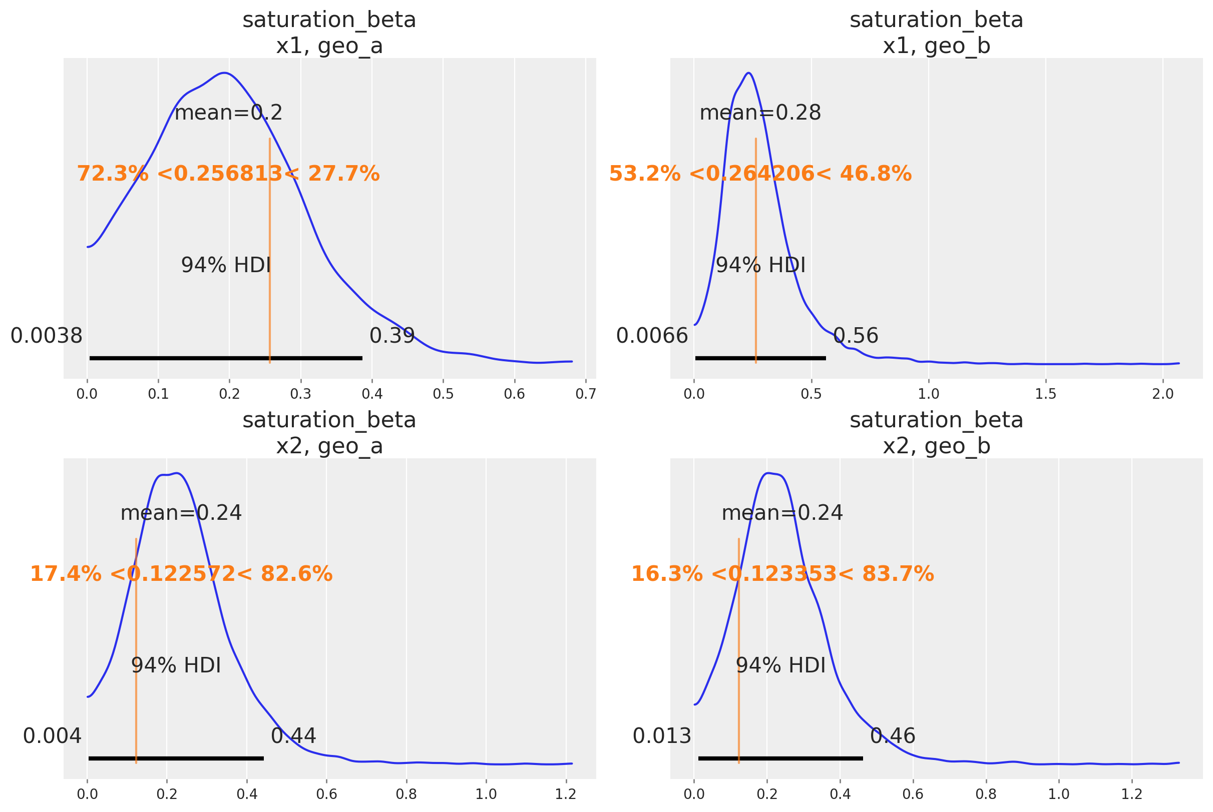
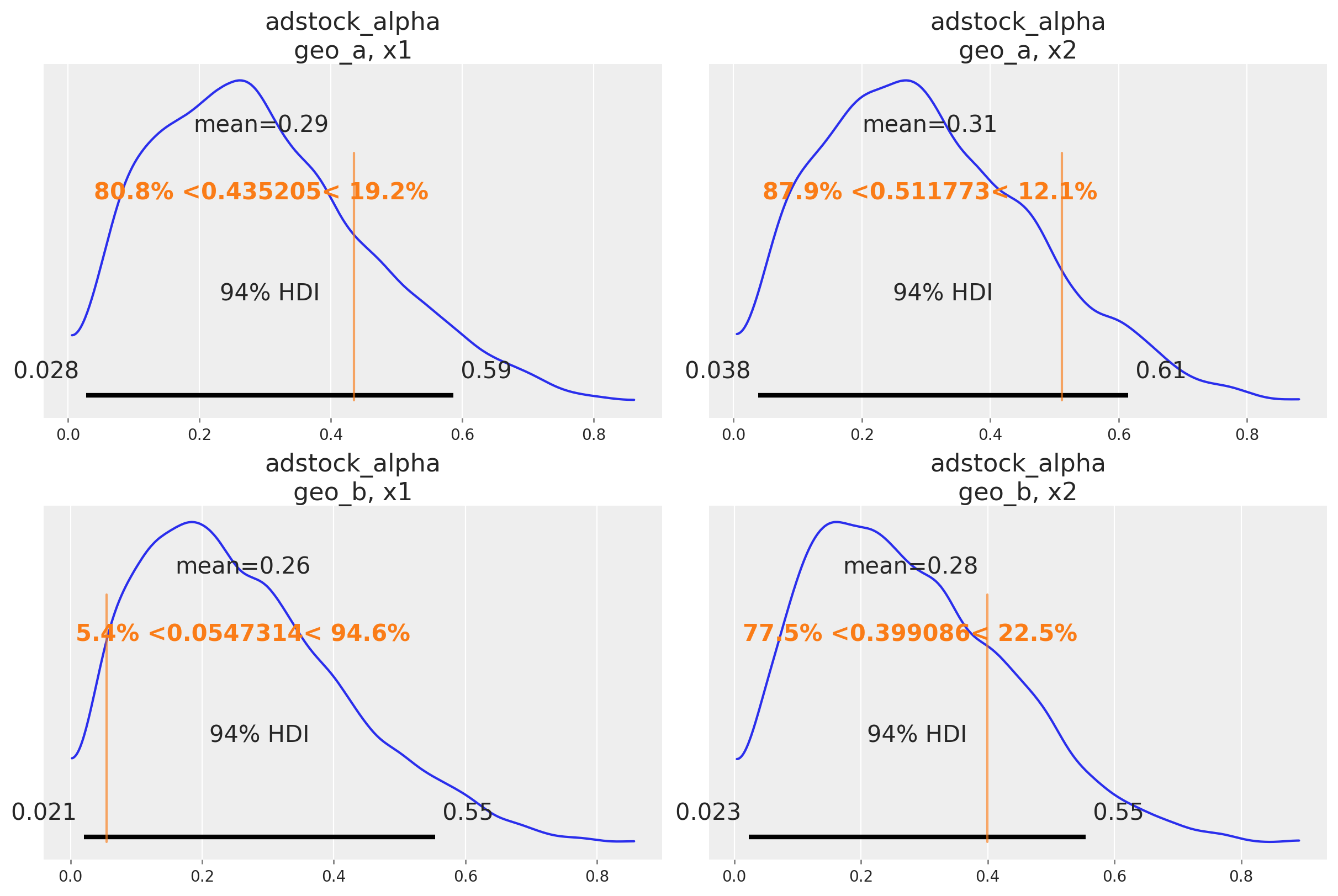
Recuperación de parámetros#
Una buena señal de que el modelo funciona como se pretende es que puede recuperar los valores verdaderos de los parámetros subyacentes al mecanismo de marketing. En nuestro caso, conocemos los valores verdaderos de los parámetros porque simulamos los datos. De forma informal, si la mayor parte de la distribución posterior cubre el valor del parámetro, es una buena señal. No esperamos que la media de la posterior siempre coincida con el valor verdadero: para datos pequeños o ruidosos, deberíamos esperar que la posterior cubra un intervalo amplio independientemente de si construimos un buen modelo o no. También existen marcos formales para pensar sobre la recuperación de parámetros en simulaciones que pueden ser útiles si necesitas evidencia aún más rigurosa de que el modelo funciona correctamente.
A continuación comparamos la distribución posterior con los valores verdaderos de los principales parámetros del MMM (saturation lambda, saturation beta y adstock alpha).
# Load the true parameters used to generate the data

data_path = data_dir / "mmm_multidimensional_example_true_parameters.nc"
true_parameters = xr.open_dataset(data_path)
az.plot_posterior(
    mmm.fit_result,
    var_names=[
        "saturation_lam",
    ],
    figsize=(12, 4),
    ref_val={
        "saturation_lam": [
            {
                "channel": "x1",
                "ref_val": true_parameters["saturation_lam"].sel(channel="x1").values,
            },
            {
                "channel": "x2",
                "ref_val": true_parameters["saturation_lam"].sel(channel="x2").values,
            },
        ]
    },
);
az.plot_posterior(
    mmm.fit_result,
    var_names=[
        "saturation_beta",
    ],
    grid=(2, 2),
    figsize=(12, 8),
    ref_val={
        "saturation_beta": [
            {
                "channel": "x1",
                "geo": "geo_a",
                "ref_val": true_parameters["saturation_beta"]
                .sel(channel="x1", geo="geo_a")
                .values,
            },
            {
                "channel": "x2",
                "geo": "geo_a",
                "ref_val": true_parameters["saturation_beta"]
                .sel(channel="x2", geo="geo_a")
                .values,
            },
            {
                "channel": "x1",
                "geo": "geo_b",
                "ref_val": true_parameters["saturation_beta"]
                .sel(channel="x1", geo="geo_b")
                .values,
            },
            {
                "channel": "x2",
                "geo": "geo_b",
                "ref_val": true_parameters["saturation_beta"]
                .sel(channel="x2", geo="geo_b")
                .values,
            },
        ]
    },
);
az.plot_posterior(
    mmm.fit_result,
    var_names=[
        "adstock_alpha",
    ],
    grid=(2, 2),
    figsize=(12, 8),
    ref_val={
        "adstock_alpha": [
            {
                "channel": "x1",
                "geo": "geo_a",
                "ref_val": true_parameters["adstock_alpha"]
                .sel(channel="x1", geo="geo_a")
                .values,
            },
            {
                "channel": "x2",
                "geo": "geo_a",
                "ref_val": true_parameters["adstock_alpha"]
                .sel(channel="x2", geo="geo_a")
                .values,
            },
            {
                "channel": "x1",
                "geo": "geo_b",
                "ref_val": true_parameters["adstock_alpha"]
                .sel(channel="x1", geo="geo_b")
                .values,
            },
            {
                "channel": "x2",
                "geo": "geo_b",
                "ref_val": true_parameters["adstock_alpha"]
                .sel(channel="x2", geo="geo_b")
                .values,
            },
        ]
    },
);
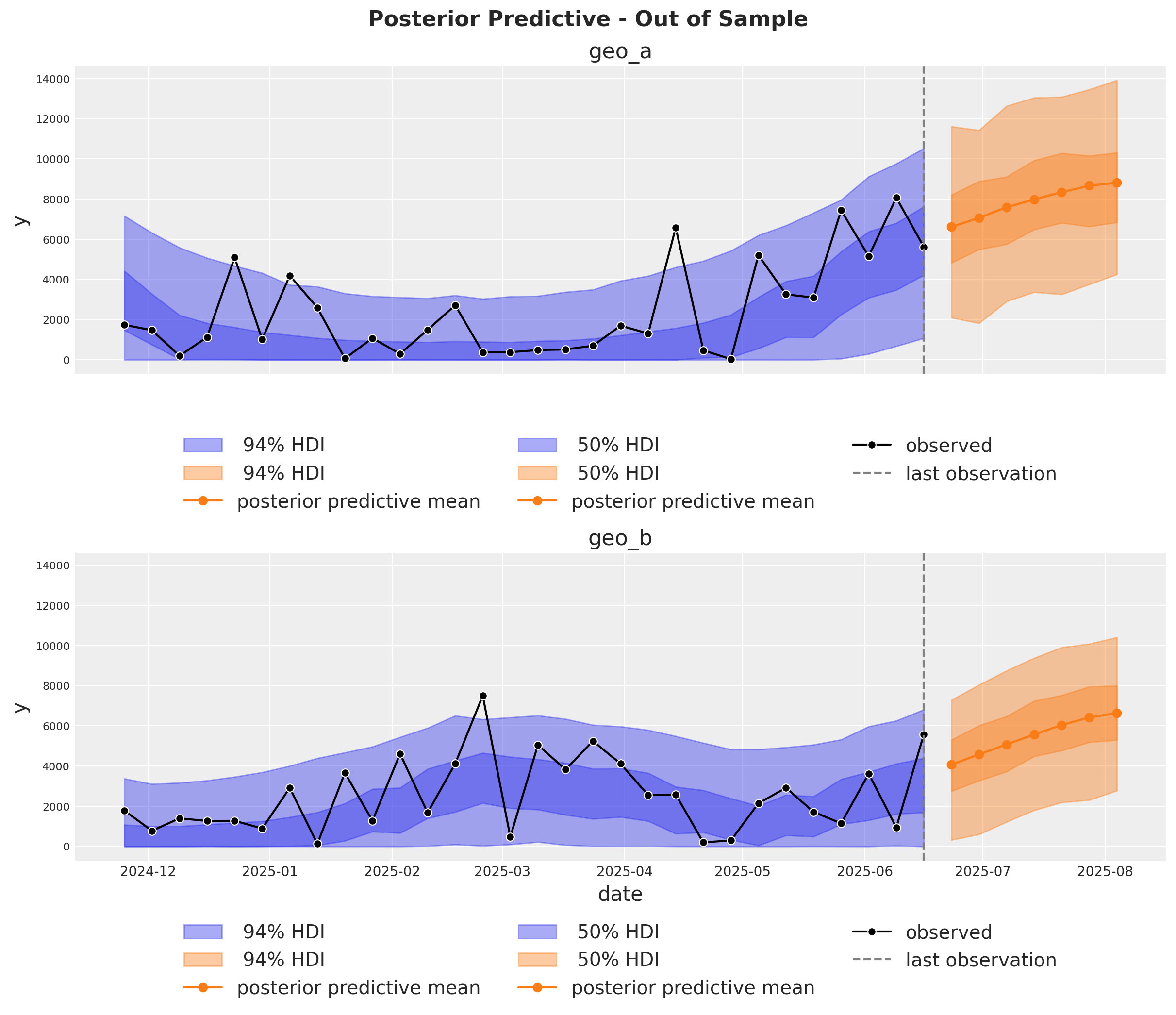
Predicciones fuera de muestra#
Es muy importante poder hacer predicciones fuera de la muestra. Esto es clave para la validación del modelo, la planificación de escenarios prospectivos y la toma de decisiones empresariales. De forma similar a Cuaderno de ejemplo para MMM, asumimos que las inversiones futuras son las mismas que el último día de la muestra de entrenamiento. De este modo podemos crear un nuevo dataset con las fechas futuras y los gastos por canal y usar el modelo para hacer predicciones.
last_date = x_train["date"].max()

# New dates starting from last in dataset
n_new = 7
new_dates = pd.date_range(start=last_date, periods=1 + n_new, freq="W-MON")[1:]

x_out_of_sample_geo_a = pd.DataFrame({"date": new_dates, "geo": "geo_a"})
x_out_of_sample_geo_b = pd.DataFrame({"date": new_dates, "geo": "geo_b"})

# Same channel spends as last day
x_out_of_sample_geo_a["x1"] = x_train.query("geo == 'geo_a'")["x1"].iloc[-1]
x_out_of_sample_geo_a["x2"] = x_train.query("geo == 'geo_a'")["x2"].iloc[-1]

x_out_of_sample_geo_b["x1"] = x_train.query("geo == 'geo_b'")["x1"].iloc[-1]
x_out_of_sample_geo_b["x2"] = x_train.query("geo == 'geo_b'")["x2"].iloc[-1]

# Other features
## Event 1
x_out_of_sample_geo_a["event_1"] = 0.0
x_out_of_sample_geo_a["event_2"] = 0.0
## Event 2
x_out_of_sample_geo_b["event_1"] = 0.0
x_out_of_sample_geo_b["event_2"] = 0.0

x_out_of_sample = pd.concat([x_out_of_sample_geo_a, x_out_of_sample_geo_b])

# Final dataset to generate out of sample predictions.
x_out_of_sample
| date | geo | x1 | x2 | event_1 | event_2 | |
|---|---|---|---|---|---|---|
| 0 | 2025-06-23 | geo_a | 0.0 | 6384.065021 | 0.0 | 0.0 |
| 1 | 2025-06-30 | geo_a | 0.0 | 6384.065021 | 0.0 | 0.0 |
| 2 | 2025-07-07 | geo_a | 0.0 | 6384.065021 | 0.0 | 0.0 |
| 3 | 2025-07-14 | geo_a | 0.0 | 6384.065021 | 0.0 | 0.0 |
| 4 | 2025-07-21 | geo_a | 0.0 | 6384.065021 | 0.0 | 0.0 |
| 5 | 2025-07-28 | geo_a | 0.0 | 6384.065021 | 0.0 | 0.0 |
| 6 | 2025-08-04 | geo_a | 0.0 | 6384.065021 | 0.0 | 0.0 |
| 0 | 2025-06-23 | geo_b | 0.0 | 8090.900533 | 0.0 | 0.0 |
| 1 | 2025-06-30 | geo_b | 0.0 | 8090.900533 | 0.0 | 0.0 |
| 2 | 2025-07-07 | geo_b | 0.0 | 8090.900533 | 0.0 | 0.0 |
| 3 | 2025-07-14 | geo_b | 0.0 | 8090.900533 | 0.0 | 0.0 |
| 4 | 2025-07-21 | geo_b | 0.0 | 8090.900533 | 0.0 | 0.0 |
| 5 | 2025-07-28 | geo_b | 0.0 | 8090.900533 | 0.0 | 0.0 |
| 6 | 2025-08-04 | geo_b | 0.0 | 8090.900533 | 0.0 | 0.0 |
Usando el mismo método sample_posterior_predictive, ahora podemos generar el pronóstico.
y_out_of_sample = mmm.sample_posterior_predictive(
    x_out_of_sample,
    extend_idata=False,
    include_last_observations=True,
    random_seed=rng,
    var_names=["y_original_scale"],
)

y_out_of_sample
Sampling: [y]
<xarray.Dataset> Size: 544kB
Dimensions:           (date: 7, geo: 2, sample: 4000)
Coordinates:
  * date              (date) datetime64[ns] 56B 2025-06-23 ... 2025-08-04
  * geo               (geo) <U5 40B 'geo_a' 'geo_b'
  * sample            (sample) object 32kB MultiIndex
  * chain             (sample) int64 32kB 0 0 0 0 0 0 0 0 0 ... 3 3 3 3 3 3 3 3
  * draw              (sample) int64 32kB 0 1 2 3 4 5 ... 995 996 997 998 999
Data variables:
    y_original_scale  (date, geo, sample) float64 448kB 7.215e+03 ... 6.687e+03
Attributes:
    created_at:                 2026-01-26T15:51:31.302277+00:00
    arviz_version:              0.23.0
    inference_library:          pymc
inference_library_version: 5.27.0fig, axes = plt.subplots(
nrows=2,
ncols=1,
figsize=(12, 10),
sharex=True,
sharey=True,
layout="constrained",
)
n_train_to_plot = 30
for ax, geo in zip(axes, mmm.model.coords["geo"], strict=True):
for hdi_prob in [0.94, 0.5]:
az.plot_hdi(
x=mmm.model.coords["date"][-n_train_to_plot:],
y=(
mmm.idata["posterior_predictive"].y_original_scale.sel(geo=geo)[
:, :, -n_train_to_plot:
]
),
color="C0",
smooth=False,
hdi_prob=hdi_prob,
fill_kwargs={"alpha": 0.4, "label": f"{hdi_prob: 0.0%} HDI"},
ax=ax,
)
az.plot_hdi(
x_out_of_sample.query("geo == @geo")["date"],
(
y_out_of_sample["y_original_scale"]
.sel(geo=geo)
.unstack()
.transpose(..., "date")
),
color="C1",
smooth=False,
hdi_prob=hdi_prob,
fill_kwargs={"alpha": 0.4, "label": f"{hdi_prob: 0.0%} HDI"},
ax=ax,
)
ax.plot(
x_out_of_sample.query("geo == @geo")["date"],
y_out_of_sample["y_original_scale"].sel(geo=geo).mean(dim="sample"),
marker="o",
color="C1",
label="posterior predictive mean",
)
sns.lineplot(
data=data_df.query("(geo == @geo)").tail(n_train_to_plot),
x="date",
y="y",
marker="o",
color="black",
label="observed",
ax=ax,
)
ax.axvline(x=last_date, color="gray", linestyle="--", label="last observation")
ax.legend(
loc="upper center",
bbox_to_anchor=(0.5, -0.15),
ncol=3,
)
ax.set(title=f"{geo}")
fig.suptitle(
"Posterior Predictive - Out of Sample", fontsize=16, fontweight="bold", y=1.03
);
Optimización#
Si quieres ejecutar optimizaciones, entonces necesitas usar MultiDimensionalBudgetOptimizerWrapper.
optimizable_model = MultiDimensionalBudgetOptimizerWrapper(
    model=mmm, start_date="2021-10-01", end_date="2021-12-31"
)

allocation_xarray, scipy_opt_result = optimizable_model.optimize_budget(
    budget=100_000,
)

sample_allocation = optimizable_model.sample_response_distribution(
    allocation_strategy=allocation_xarray,
)
Sampling: [y]
¡Este objeto es un dataset de xarray con la asignación y las respuestas predictivas posteriores!
sample_allocation
<xarray.Dataset> Size: 4MB
Dimensions:                                  (date: 21, geo: 2, channel: 2,
                                              sample: 4000)
Coordinates:
  * date                                     (date) datetime64[ns] 168B 2021-...
  * geo                                      (geo) <U5 40B 'geo_a' 'geo_b'
  * channel                                  (channel) <U2 16B 'x1' 'x2'
  * sample                                   (sample) object 32kB MultiIndex
  * chain                                    (sample) int64 32kB 0 0 0 ... 3 3 3
  * draw                                     (sample) int64 32kB 0 1 ... 998 999
Data variables:
    channel_contribution                     (date, geo, channel, sample) float64 3MB ...
    total_media_contribution_original_scale  (sample) float64 32kB 6.329e+04 ...
    y                                        (date, geo, sample) float64 1MB ...
    allocation                               (geo, channel) float64 32B 2.414...
    x1                                       (date, geo) float64 336B 2.415e+...
    x2                                       (date, geo) float64 336B 3.05e+0...
Attributes:
    created_at:                 2026-01-26T15:51:35.610974+00:00
    arviz_version:              0.23.0
    inference_library:          pymc
inference_library_version: 5.27.0Una vez obtengas la asignación, puedes graficar los resultados 🚀
optimizable_model.plot.budget_allocation(
    samples=sample_allocation,
);
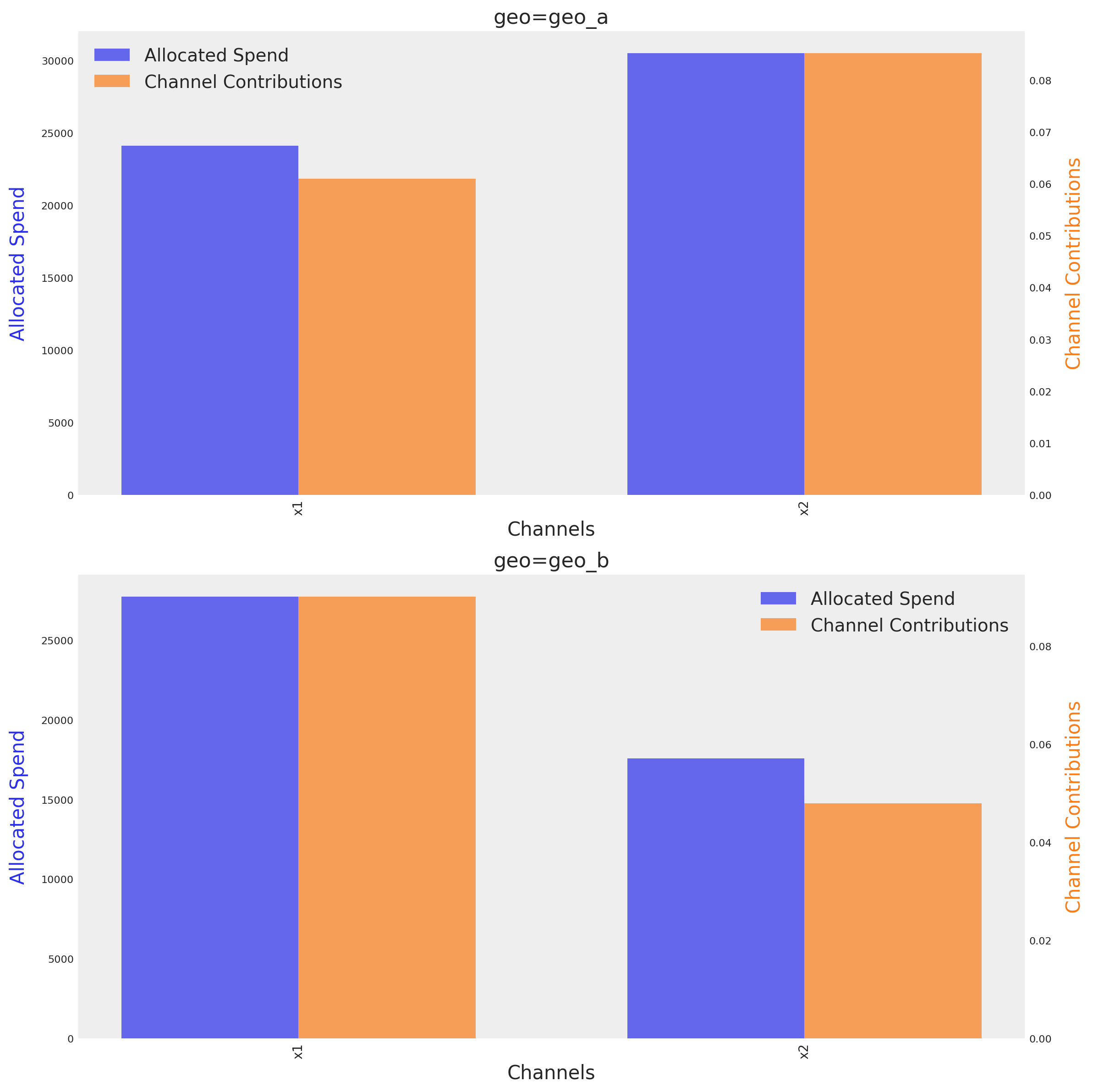
El gráfico muestra el presupuesto óptimo para cada canal en cada geo, junto a su contribución media respectiva dado el presupuesto óptimo. El método identifica automáticamente el número de dimensiones e intenta crear una gráfica en función de ellas.
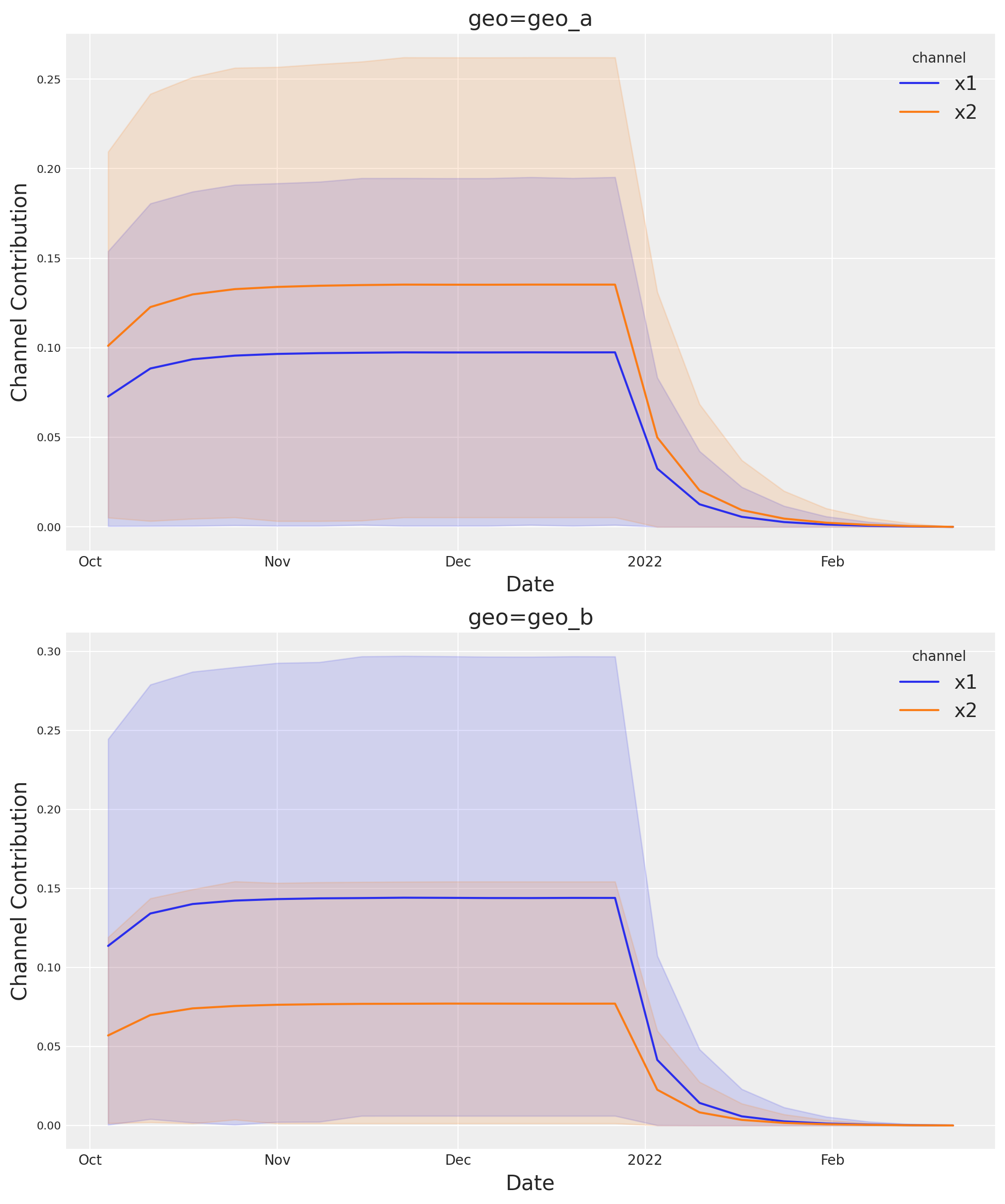
Si quieres ver la incertidumbre completa a lo largo del tiempo, puedes usar la suite de gráficos y el método allocated_contribution_by_channel_over_time.
optimizable_model.plot.allocated_contribution_by_channel_over_time(
    samples=sample_allocation,
);
Si tienes un modelo personalizado, puedes envolverlo en el protocolo del modelo y usar el optimizador después. Si tu modelo gestiona las escalas internamente, no necesitas modificar nada. De lo contrario, para las gráficas, quizá quieras usar scale_factor=N. Por ejemplo:
optimizable_model.plot.budget_allocation(
    samples=sample_allocation,
    scale_factor=120
);
Guardar modelo#
Opcionalmente puedes guardar el resultado de tu trabajo. Los objetos de resultados del modelo (idata) pueden volverse muy grandes cuando empezamos a trabajar en múltiples dimensiones. Por ello, a veces puede ser útil comprimir el idata antes de guardarlo. A continuación hay un par de trucos.
# Reduce your posterior (optional)
# clone_idata = mmm.idata.copy()
# clone_idata.posterior = clone_idata.posterior.astype(np.float32)
# clone_idata.posterior = clone_idata.posterior.sel(draw=slice(None, None, 10))

# clone_idata.to_netcdf("multidimensional_model_compressed.nc", groups=["posterior", "fit_data"], engine="h5netcdf")
Nota
Estamos muy entusiasmados con esta nueva funcionalidad y las posibilidades que abre. ¡Esperamos tus comentarios!
%load_ext watermark
%watermark -n -u -v -iv -w -p pymc_marketing,pytensor,nutpie
Last updated: Mon, 26 Jan 2026

Python implementation: CPython
Python version       : 3.13.11
IPython version      : 9.9.0

pymc_marketing: 0.17.1
pytensor      : 2.36.3
nutpie        : 0.16.4

arviz         : 0.23.0
matplotlib    : 3.10.8
numpy         : 2.3.5
pandas        : 2.3.3
pymc          : 5.27.0
pymc_extras   : 0.7.0
pymc_marketing: 0.17.1
seaborn       : 0.13.2
xarray        : 2025.12.0

Watermark: 2.6.0