Developer Gamma-gamma model PyMC implementation

Reference:Fader, P. S., & Hardie, B. G. (2013). The Gamma-Gamma model of monetary value. February, 2, 1-9.

http://www.brucehardie.com/notes/025/gamma_gamma.pdf

import arviz as az
import matplotlib.pyplot as plt
import numpy as np
import pandas as pd
import pymc as pm
import pytensor.tensor as pt
import seaborn as sns

from pymc_marketing import clv

Simulate data

rng = np.random.default_rng(42)

# Hyperparameters
p_true = 6.
q_true = 4.
v_true = 15.

# Number of subjects
N = 500  
# Subject level parameters
nu_true = pm.draw(pm.Gamma.dist(q_true, v_true, size=N), random_seed=rng)

# Number of observations per subject
x = rng.poisson(lam=2, size=N) + 1  
idx = np.repeat(np.arange(0, N), x)
# Observations
z = pm.draw(pm.Gamma.dist(p_true, nu_true[idx]), random_seed=rng)

print(sum(x))
assert len(nu_true[idx]) == sum(x)

1503

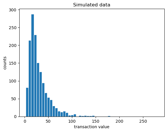
plt.hist(z, bins=50, ec="w")
plt.xlabel("transaction value")
plt.ylabel("counts")
plt.title("Simulated data");

df = pd.DataFrame(data={"individual_transaction_value": z, "customer_id": idx})
z_mean = df.groupby("customer_id").mean()["individual_transaction_value"].values
z_mean[:10]

array([ 17.5597973 ,  41.05272046,  15.90609488,  83.95307047,
        20.36896009,  23.8572992 ,  46.09000842,  47.49876237,
       131.16095313,  16.42659393])

PyMC implementation

We can use the pre-built PyMMMC implementation of the Gamma-Gamma model, which also provides nice ploting and prediction methods

Using individual transactions 𝑧

model = clv.GammaGammaModelIndividual(data = df)

model

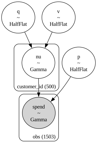
Gamma-Gamma Model (Individual Transactions)
    p ~ HalfFlat()
    q ~ HalfFlat()
    v ~ HalfFlat()
   nu ~ Gamma(q, f(v))
spend ~ Gamma(p, f(nu))

model.build_model()
model.graphviz()

model.fit(random_seed=rng)

Auto-assigning NUTS sampler...
Initializing NUTS using jitter+adapt_diag...
Multiprocess sampling (4 chains in 4 jobs)
NUTS: [p, q, v, nu]

100.00% [8000/8000 00:15<00:00 Sampling 4 chains, 0 divergences]

Sampling 4 chains for 1_000 tune and 1_000 draw iterations (4_000 + 4_000 draws total) took 16 seconds.

arviz.InferenceData

• posterior

  <xarray.Dataset>
  Dimensions:      (chain: 4, draw: 1000, customer_id: 500)
  Coordinates:
    * chain        (chain) int64 0 1 2 3
    * draw         (draw) int64 0 1 2 3 4 5 6 7 ... 993 994 995 996 997 998 999
    * customer_id  (customer_id) int64 0 1 2 3 4 5 6 ... 494 495 496 497 498 499
  Data variables:
      p            (chain, draw) float64 6.043 6.218 6.028 ... 5.783 5.617 5.341
      q            (chain, draw) float64 3.977 4.26 3.962 ... 4.277 4.209 3.401
      v            (chain, draw) float64 14.94 15.73 15.36 ... 18.15 18.12 14.57
      nu           (chain, draw, customer_id) float64 0.204 0.1759 ... 0.1358
  Attributes:
      created_at:                 2022-12-15T08:50:41.657496
      arviz_version:              0.14.0
      inference_library:          pymc
      inference_library_version:  5.0.0
      sampling_time:              15.84934139251709
      tuning_steps:               1000

  xarray.Dataset

  • Dimensions:
    • chain: 4
    • draw: 1000
    • customer_id: 500
  • Coordinates: (3)
    • chain
      (chain)
      int64
      0 1 2 3

      array([0, 1, 2, 3])

    • draw
      (draw)
      int64
      0 1 2 3 4 5 ... 995 996 997 998 999

      array([  0,   1,   2, ..., 997, 998, 999])

    • customer_id
      (customer_id)
      int64
      0 1 2 3 4 5 ... 495 496 497 498 499

      array([  0,   1,   2, ..., 497, 498, 499])

  • Data variables: (4)
    • p
      (chain, draw)
      float64
      6.043 6.218 6.028 ... 5.617 5.341

      array([[6.04327463, 6.21762803, 6.02827294, ..., 5.80928028, 5.79542957,
              5.75397046],
             [5.94612405, 6.02720383, 6.09979741, ..., 6.25592877, 6.23107604,
              6.31658144],
             [6.04863789, 5.9324924 , 6.06681277, ..., 5.93310676, 5.97014969,
              6.03208966],
             [6.01556719, 6.07452861, 6.08100824, ..., 5.7831662 , 5.61669483,
              5.34064114]])

    • q
      (chain, draw)
      float64
      3.977 4.26 3.962 ... 4.209 3.401

      array([[3.97742158, 4.2597312 , 3.96202545, ..., 3.94381452, 3.66760917,
              3.93359479],
             [4.01548967, 3.73011515, 3.84946458, ..., 3.77171431, 3.84029333,
              3.98255855],
             [3.5910417 , 4.23155088, 3.54007528, ..., 3.8940765 , 4.16368899,
              4.35897785],
             [3.94408973, 3.60495415, 4.69175689, ..., 4.27739282, 4.20865459,
              3.40125298]])

    • v
      (chain, draw)
      float64
      14.94 15.73 15.36 ... 18.12 14.57

      array([[14.94271866, 15.72971931, 15.36417589, ..., 15.00717933,
              15.55705697, 15.85005664],
             [15.19790784, 14.28127672, 14.85818201, ..., 13.63812327,
              14.05452379, 14.56003244],
             [13.82164922, 16.65928378, 13.39669299, ..., 15.09649916,
              16.237263  , 16.2283887 ],
             [15.20300646, 14.12626531, 17.91131214, ..., 18.1536756 ,
              18.12446886, 14.56999038]])

    • nu
      (chain, draw, customer_id)
      float64
      0.204 0.1759 ... 0.6245 0.1358

      array([[[0.20404515, 0.17594074, 0.34814799, ..., 0.39091135,
               0.5003159 , 0.1365436 ],
              [0.43004694, 0.14350215, 0.32756627, ..., 0.33614911,
               0.82772329, 0.17282259],
              [0.30179892, 0.12126385, 0.37631443, ..., 0.31019172,
               0.48542782, 0.18584842],
              ...,
              [0.28951152, 0.18270745, 0.32002249, ..., 0.30891873,
               0.83532785, 0.15244004],
              [0.27900133, 0.16165941, 0.32445352, ..., 0.30164199,
               0.75770934, 0.11884918],
              [0.35666248, 0.143205  , 0.33165941, ..., 0.37146942,
               0.49968217, 0.23305084]],
      
             [[0.33065761, 0.10885326, 0.44750507, ..., 0.43843246,
               0.72155734, 0.12956621],
              [0.2571464 , 0.16186308, 0.2686646 , ..., 0.42677421,
               0.71518814, 0.23231473],
              [0.42074619, 0.16861043, 0.42408696, ..., 0.28849036,
               0.60320519, 0.1518702 ],
      ...
              [0.31438148, 0.1228502 , 0.36378012, ..., 0.26075103,
               0.88791443, 0.13435966],
              [0.27312207, 0.19957795, 0.28659475, ..., 0.29807603,
               0.72405137, 0.16011446],
              [0.31329891, 0.13277298, 0.5293466 , ..., 0.2990259 ,
               0.75169844, 0.21487413]],
      
             [[0.38888388, 0.19041862, 0.4426441 , ..., 0.32773927,
               0.54546591, 0.19509514],
              [0.53477945, 0.18882481, 0.44027482, ..., 0.32627763,
               0.6596879 , 0.21921767],
              [0.18638001, 0.13243787, 0.29068887, ..., 0.34788272,
               0.67172601, 0.14216851],
              ...,
              [0.31136407, 0.15573123, 0.23187793, ..., 0.30662508,
               0.71338544, 0.14903962],
              [0.28770619, 0.13976676, 0.42298707, ..., 0.33185163,
               0.45927597, 0.16525165],
              [0.31629331, 0.14071874, 0.19703696, ..., 0.30999261,
               0.6245466 , 0.13575634]]])

  • Indexes: (3)
    • chain
      PandasIndex

      PandasIndex(Int64Index([0, 1, 2, 3], dtype='int64', name='chain'))

    • draw
      PandasIndex

      PandasIndex(Int64Index([  0,   1,   2,   3,   4,   5,   6,   7,   8,   9,
                  ...
                  990, 991, 992, 993, 994, 995, 996, 997, 998, 999],
                 dtype='int64', name='draw', length=1000))

    • customer_id
      PandasIndex

      PandasIndex(Int64Index([  0,   1,   2,   3,   4,   5,   6,   7,   8,   9,
                  ...
                  490, 491, 492, 493, 494, 495, 496, 497, 498, 499],
                 dtype='int64', name='customer_id', length=500))

  • Attributes: (6)

    created_at :

    2022-12-15T08:50:41.657496

    arviz_version :

    0.14.0

    inference_library :

    pymc

    inference_library_version :

    5.0.0

    sampling_time :

    15.84934139251709

    tuning_steps :

    1000

  
  
• sample_stats

  <xarray.Dataset>
  Dimensions:                (chain: 4, draw: 1000)
  Coordinates:
    * chain                  (chain) int64 0 1 2 3
    * draw                   (draw) int64 0 1 2 3 4 5 ... 994 995 996 997 998 999
  Data variables: (12/17)
      n_steps                (chain, draw) float64 15.0 15.0 15.0 ... 15.0 15.0
      max_energy_error       (chain, draw) float64 0.6677 -0.3882 ... -1.41 1.565
      lp                     (chain, draw) float64 -5.977e+03 ... -6.014e+03
      process_time_diff      (chain, draw) float64 0.005394 0.004418 ... 0.006559
      tree_depth             (chain, draw) int64 4 4 4 4 4 4 4 4 ... 4 4 4 4 4 4 4
      index_in_trajectory    (chain, draw) int64 8 -9 -6 3 -6 ... 9 -3 -7 11 -13
      ...                     ...
      energy                 (chain, draw) float64 6.208e+03 ... 6.283e+03
      perf_counter_start     (chain, draw) float64 2.382e+03 ... 2.387e+03
      reached_max_treedepth  (chain, draw) bool False False False ... False False
      acceptance_rate        (chain, draw) float64 0.6662 0.9528 ... 0.9918 0.559
      step_size_bar          (chain, draw) float64 0.2451 0.2451 ... 0.2524 0.2524
      step_size              (chain, draw) float64 0.2618 0.2618 ... 0.2271 0.2271
  Attributes:
      created_at:                 2022-12-15T08:50:41.673955
      arviz_version:              0.14.0
      inference_library:          pymc
      inference_library_version:  5.0.0
      sampling_time:              15.84934139251709
      tuning_steps:               1000

  xarray.Dataset

  • Dimensions:
    • chain: 4
    • draw: 1000
  • Coordinates: (2)
    • chain
      (chain)
      int64
      0 1 2 3

      array([0, 1, 2, 3])

    • draw
      (draw)
      int64
      0 1 2 3 4 5 ... 995 996 997 998 999

      array([  0,   1,   2, ..., 997, 998, 999])

  • Data variables: (17)
    • n_steps
      (chain, draw)
      float64
      15.0 15.0 15.0 ... 15.0 15.0 15.0

      array([[15., 15., 15., ..., 15., 15., 15.],
             [15., 15., 15., ..., 15., 15., 15.],
             [15., 15., 15., ..., 15., 15., 15.],
             [15., 15., 15., ..., 15., 15., 15.]])

    • max_energy_error
      (chain, draw)
      float64
      0.6677 -0.3882 ... -1.41 1.565

      array([[ 0.66774509, -0.38817184,  0.59953829, ...,  1.23805773,
               1.71308259, -0.99475154],
             [-0.6798151 , -0.43840712,  0.53033489, ..., -0.70938027,
              -0.72497306,  0.75226713],
             [ 0.54401806,  0.38771646,  0.52059962, ...,  1.08943729,
               0.59963789,  0.67391278],
             [ 4.30059989,  1.19783192, -1.12160454, ..., -1.13836277,
              -1.41038285,  1.56487068]])

    • lp
      (chain, draw)
      float64
      -5.977e+03 ... -6.014e+03

      array([[-5977.29221356, -5957.8528124 , -5996.04904321, ...,
              -5988.32680757, -6007.37122464, -6000.9319408 ],
             [-5995.36783863, -6004.5170187 , -6011.51185314, ...,
              -6007.78309957, -5975.26058928, -5966.91294951],
             [-5997.59508452, -5998.68225118, -6008.88478588, ...,
              -6001.04463324, -5994.47205083, -5999.77921559],
             [-5988.9680808 , -5976.39798022, -5970.79693241, ...,
              -6003.36585324, -5996.51178553, -6014.10939495]])

    • process_time_diff
      (chain, draw)
      float64
      0.005394 0.004418 ... 0.006559

      array([[0.00539355, 0.00441797, 0.00486682, ..., 0.00439751, 0.00396931,
              0.00372992],
             [0.00447363, 0.00398174, 0.00449191, ..., 0.00396219, 0.00395491,
              0.00385809],
             [0.00454427, 0.00453113, 0.00425225, ..., 0.00459463, 0.00399573,
              0.00410339],
             [0.00521637, 0.00510699, 0.00420741, ..., 0.00560952, 0.00678979,
              0.0065586 ]])

    • tree_depth
      (chain, draw)
      int64
      4 4 4 4 4 4 4 4 ... 4 4 4 4 4 4 4 4

      array([[4, 4, 4, ..., 4, 4, 4],
             [4, 4, 4, ..., 4, 4, 4],
             [4, 4, 4, ..., 4, 4, 4],
             [4, 4, 4, ..., 4, 4, 4]])

    • index_in_trajectory
      (chain, draw)
      int64
      8 -9 -6 3 -6 -9 ... 9 -3 -7 11 -13

      array([[  8,  -9,  -6, ...,   9,   3,  12],
             [  1,  -7, -12, ...,   9,  -7,  -3],
             [-14,   9, -12, ...,   8,   5,  -6],
             [  2,   4,  13, ...,  -7,  11, -13]])

    • largest_eigval
      (chain, draw)
      float64
      nan nan nan nan ... nan nan nan nan

      array([[nan, nan, nan, ..., nan, nan, nan],
             [nan, nan, nan, ..., nan, nan, nan],
             [nan, nan, nan, ..., nan, nan, nan],
             [nan, nan, nan, ..., nan, nan, nan]])

    • smallest_eigval
      (chain, draw)
      float64
      nan nan nan nan ... nan nan nan nan

      array([[nan, nan, nan, ..., nan, nan, nan],
             [nan, nan, nan, ..., nan, nan, nan],
             [nan, nan, nan, ..., nan, nan, nan],
             [nan, nan, nan, ..., nan, nan, nan]])

    • energy_error
      (chain, draw)
      float64
      0.3048 -0.06628 ... -0.439 1.156

      array([[ 0.30477068, -0.06627895,  0.56421703, ...,  0.58543563,
               0.53386245, -0.99475154],
             [ 0.11468303, -0.03931299,  0.36164668, ..., -0.06267336,
              -0.65809512, -0.2440443 ],
             [ 0.22164835,  0.04621575,  0.28026599, ...,  0.41861985,
              -0.11415979,  0.30923898],
             [-0.59671797,  0.44887144, -1.0403743 , ...,  0.05597321,
              -0.43904087,  1.15622433]])

    • perf_counter_diff
      (chain, draw)
      float64
      0.005401 0.004417 ... 0.006568

      array([[0.00540106, 0.00441668, 0.00487192, ..., 0.00448029, 0.00405588,
              0.00381165],
             [0.00447281, 0.00399035, 0.00449062, ..., 0.00396871, 0.00395394,
              0.00386428],
             [0.0045438 , 0.00452977, 0.00425899, ..., 0.0046011 , 0.00399535,
              0.00411162],
             [0.00521649, 0.00512552, 0.00429714, ..., 0.00561689, 0.00679984,
              0.00656804]])

    • diverging
      (chain, draw)
      bool
      False False False ... False False

      array([[False, False, False, ..., False, False, False],
             [False, False, False, ..., False, False, False],
             [False, False, False, ..., False, False, False],
             [False, False, False, ..., False, False, False]])

    • energy
      (chain, draw)
      float64
      6.208e+03 6.195e+03 ... 6.283e+03

      array([[6207.86055093, 6194.78836348, 6216.24844567, ..., 6246.04936045,
              6249.13859346, 6270.94041853],
             [6219.5165432 , 6241.94020777, 6260.57519425, ..., 6245.38071535,
              6242.56161635, 6237.02700357],
             [6259.88673605, 6232.38784001, 6241.83052136, ..., 6245.85422515,
              6262.75146149, 6255.69971649],
             [6228.16205248, 6232.99284301, 6206.53859292, ..., 6253.83640973,
              6226.67815788, 6283.44954109]])

    • perf_counter_start
      (chain, draw)
      float64
      2.382e+03 2.382e+03 ... 2.387e+03

      array([[2381.82289778, 2381.82852162, 2381.83316733, ..., 2386.98022534,
              2386.98491888, 2386.98916539],
             [2381.44610395, 2381.45079892, 2381.45498343, ..., 2386.47216313,
              2386.4763171 , 2386.48047381],
             [2381.16174944, 2381.16650705, 2381.17127485, ..., 2386.15528356,
              2386.16012141, 2386.16433028],
             [2382.24056807, 2382.24607918, 2382.25140763, ..., 2387.20138177,
              2387.20739462, 2387.21449516]])

    • reached_max_treedepth
      (chain, draw)
      bool
      False False False ... False False

      array([[False, False, False, ..., False, False, False],
             [False, False, False, ..., False, False, False],
             [False, False, False, ..., False, False, False],
             [False, False, False, ..., False, False, False]])

    • acceptance_rate
      (chain, draw)
      float64
      0.6662 0.9528 ... 0.9918 0.559

      array([[0.6661684 , 0.95275493, 0.75495822, ..., 0.69334442, 0.6967956 ,
              0.88606517],
             [0.99030257, 0.97444655, 0.78880395, ..., 0.94446593, 0.97202581,
              0.81527745],
             [0.76174013, 0.92765456, 0.85133663, ..., 0.58376679, 0.83357172,
              0.7470202 ],
             [0.33124962, 0.60552709, 0.78098179, ..., 0.97719893, 0.99179469,
              0.55895659]])

    • step_size_bar
      (chain, draw)
      float64
      0.2451 0.2451 ... 0.2524 0.2524

      array([[0.24508299, 0.24508299, 0.24508299, ..., 0.24508299, 0.24508299,
              0.24508299],
             [0.25900637, 0.25900637, 0.25900637, ..., 0.25900637, 0.25900637,
              0.25900637],
             [0.25385358, 0.25385358, 0.25385358, ..., 0.25385358, 0.25385358,
              0.25385358],
             [0.25237677, 0.25237677, 0.25237677, ..., 0.25237677, 0.25237677,
              0.25237677]])

    • step_size
      (chain, draw)
      float64
      0.2618 0.2618 ... 0.2271 0.2271

      array([[0.26178739, 0.26178739, 0.26178739, ..., 0.26178739, 0.26178739,
              0.26178739],
             [0.22372739, 0.22372739, 0.22372739, ..., 0.22372739, 0.22372739,
              0.22372739],
             [0.24243123, 0.24243123, 0.24243123, ..., 0.24243123, 0.24243123,
              0.24243123],
             [0.22707643, 0.22707643, 0.22707643, ..., 0.22707643, 0.22707643,
              0.22707643]])

  • Indexes: (2)
    • chain
      PandasIndex

      PandasIndex(Int64Index([0, 1, 2, 3], dtype='int64', name='chain'))

    • draw
      PandasIndex

      PandasIndex(Int64Index([  0,   1,   2,   3,   4,   5,   6,   7,   8,   9,
                  ...
                  990, 991, 992, 993, 994, 995, 996, 997, 998, 999],
                 dtype='int64', name='draw', length=1000))

  • Attributes: (6)

    created_at :

    2022-12-15T08:50:41.673955

    arviz_version :

    0.14.0

    inference_library :

    pymc

    inference_library_version :

    5.0.0

    sampling_time :

    15.84934139251709

    tuning_steps :

    1000

  
  
• observed_data

  <xarray.Dataset>
  Dimensions:  (obs: 1503)
  Coordinates:
    * obs      (obs) int64 0 1 2 3 4 5 6 7 ... 1496 1497 1498 1499 1500 1501 1502
  Data variables:
      spend    (obs) float64 14.17 11.38 20.49 24.21 ... 33.88 31.51 49.41 30.51
  Attributes:
      created_at:                 2022-12-15T08:50:41.680915
      arviz_version:              0.14.0
      inference_library:          pymc
      inference_library_version:  5.0.0

  xarray.Dataset

  • Dimensions:
    • obs: 1503
  • Coordinates: (1)
    • obs
      (obs)
      int64
      0 1 2 3 4 ... 1499 1500 1501 1502

      array([   0,    1,    2, ..., 1500, 1501, 1502])

  • Data variables: (1)
    • spend
      (obs)
      float64
      14.17 11.38 20.49 ... 49.41 30.51

      array([14.16677112, 11.37667404, 20.49023511, ..., 31.50858489,
             49.40835229, 30.51465636])

  • Indexes: (1)
    • obs
      PandasIndex

      PandasIndex(Int64Index([   0,    1,    2,    3,    4,    5,    6,    7,    8,    9,
                  ...
                  1493, 1494, 1495, 1496, 1497, 1498, 1499, 1500, 1501, 1502],
                 dtype='int64', name='obs', length=1503))

  • Attributes: (4)

    created_at :

    2022-12-15T08:50:41.680915

    arviz_version :

    0.14.0

    inference_library :

    pymc

    inference_library_version :

    5.0.0

  
  

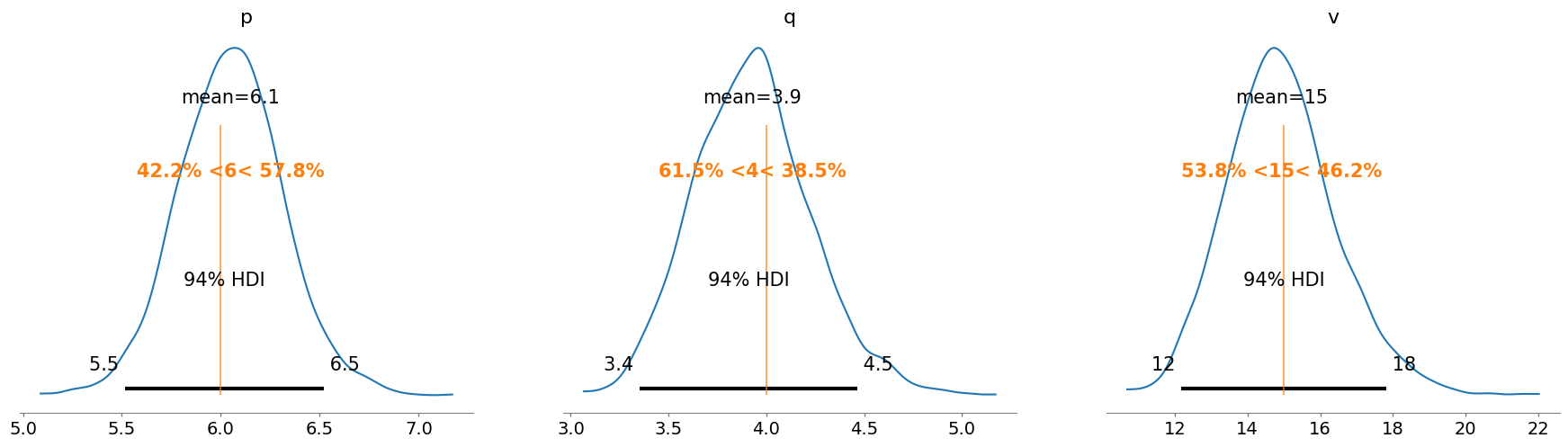
az.plot_posterior(model.fit_result, var_names=["p", "q", "v"], ref_val=[p_true, q_true, v_true]);

expected_spend = model.expected_customer_spend(
    customer_id=idx,
    individual_transaction_value=z,
).stack(sample=("draw", "chain"))

Sampling: [nu]

100.00% [4000/4000 00:00<00:00]

# Choose 10 lowest, median and 10 highest spending clients
selected_idxs = np.argsort(nu_true)[::-1][[10, 250, -10]]
selected_idxs

array([267, 407, 359])

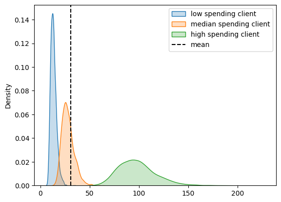
sns.kdeplot(expected_spend.sel(customer_id=selected_idxs[0]), fill=True, label="low spending client")
sns.kdeplot(expected_spend.sel(customer_id=selected_idxs[1]), fill=True, label="median spending client")
sns.kdeplot(expected_spend.sel(customer_id=selected_idxs[2]), fill=True, label="high spending client")
plt.axvline(expected_spend.mean(), color="k", ls="--", label="mean")
plt.legend();

new_spend = model.expected_new_customer_spend().stack(sample=("chain", "draw"))

Sampling: [nu]

100.00% [4000/4000 00:00<00:00]

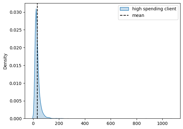
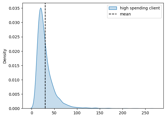
sns.kdeplot(new_spend.isel(new_customer_id=0), fill=True, label="high spending client")
plt.axvline(new_spend.mean(), color="k", ls="--", label="mean")
plt.legend();

Using average transactions per user \(\overline{z}\)

model = clv.GammaGammaModel(
    customer_id=idx,
    mean_transaction_value=z_mean,
    frequency=x,
)
model

Gamma-Gamma Model (Mean Transactions)
         p ~ HalfFlat()
         q ~ HalfFlat()
         v ~ HalfFlat()
likelihood ~ Potential(f(q, p, v))

model.fit(random_seed=rng)

Auto-assigning NUTS sampler...
Initializing NUTS using jitter+adapt_diag...
Multiprocess sampling (4 chains in 4 jobs)
NUTS: [p, q, v]

100.00% [8000/8000 00:19<00:00 Sampling 4 chains, 0 divergences]

Sampling 4 chains for 1_000 tune and 1_000 draw iterations (4_000 + 4_000 draws total) took 20 seconds.

arviz.InferenceData

• posterior

  <xarray.Dataset>
  Dimensions:  (chain: 4, draw: 1000)
  Coordinates:
    * chain    (chain) int64 0 1 2 3
    * draw     (draw) int64 0 1 2 3 4 5 6 7 8 ... 992 993 994 995 996 997 998 999
  Data variables:
      p        (chain, draw) float64 8.287 6.904 11.12 11.37 ... 5.595 7.243 5.328
      q        (chain, draw) float64 3.116 3.177 3.585 3.381 ... 3.931 3.953 3.654
      v        (chain, draw) float64 8.172 10.5 7.579 6.657 ... 16.45 12.56 15.75
  Attributes:
      created_at:                 2022-12-15T08:51:18.981662
      arviz_version:              0.14.0
      inference_library:          pymc
      inference_library_version:  5.0.0
      sampling_time:              19.611279487609863
      tuning_steps:               1000

  xarray.Dataset

  • Dimensions:
    • chain: 4
    • draw: 1000
  • Coordinates: (2)
    • chain
      (chain)
      int64
      0 1 2 3

      array([0, 1, 2, 3])

    • draw
      (draw)
      int64
      0 1 2 3 4 5 ... 995 996 997 998 999

      array([  0,   1,   2, ..., 997, 998, 999])

  • Data variables: (3)
    • p
      (chain, draw)
      float64
      8.287 6.904 11.12 ... 7.243 5.328

      array([[ 8.2872054 ,  6.90382714, 11.11879769, ...,  5.68907182,
               6.85627894,  5.96806831],
             [12.79669006,  4.84959747,  4.83463719, ...,  7.76180624,
               9.96909688,  6.49539626],
             [ 7.58104018,  6.02101377,  6.09906546, ...,  5.29522861,
               5.44120157,  6.07560515],
             [ 5.49357029,  9.28561756,  7.59296516, ...,  5.59451145,
               7.24344386,  5.32829089]])

    • q
      (chain, draw)
      float64
      3.116 3.177 3.585 ... 3.953 3.654

      array([[3.11579323, 3.1769761 , 3.58455605, ..., 3.56035428, 4.1110957 ,
              3.36723507],
             [3.22604207, 3.97993833, 3.98537764, ..., 3.21715583, 3.36359162,
              3.55841598],
             [3.84183068, 3.68841339, 4.18237521, ..., 3.67103312, 3.71839212,
              4.1324359 ],
             [3.72936092, 3.67781615, 3.50397098, ..., 3.93122875, 3.95292647,
              3.65363476]])

    • v
      (chain, draw)
      float64
      8.172 10.5 7.579 ... 12.56 15.75

      array([[ 8.17167535, 10.49600822,  7.57860713, ..., 13.71414558,
              14.36900997, 12.29861002],
             [ 5.52573168, 18.87712215, 18.73695522, ...,  9.16753387,
               7.71252211, 12.16474154],
             [11.44346793, 14.03970925, 15.95423017, ..., 15.96769078,
              15.92207223, 15.25336428],
             [15.49578399,  8.62373629, 10.40881956, ..., 16.4484807 ,
              12.55748384, 15.75406101]])

  • Indexes: (2)
    • chain
      PandasIndex

      PandasIndex(Int64Index([0, 1, 2, 3], dtype='int64', name='chain'))

    • draw
      PandasIndex

      PandasIndex(Int64Index([  0,   1,   2,   3,   4,   5,   6,   7,   8,   9,
                  ...
                  990, 991, 992, 993, 994, 995, 996, 997, 998, 999],
                 dtype='int64', name='draw', length=1000))

  • Attributes: (6)

    created_at :

    2022-12-15T08:51:18.981662

    arviz_version :

    0.14.0

    inference_library :

    pymc

    inference_library_version :

    5.0.0

    sampling_time :

    19.611279487609863

    tuning_steps :

    1000

  
  
• sample_stats

  <xarray.Dataset>
  Dimensions:                (chain: 4, draw: 1000)
  Coordinates:
    * chain                  (chain) int64 0 1 2 3
    * draw                   (draw) int64 0 1 2 3 4 5 ... 994 995 996 997 998 999
  Data variables: (12/17)
      n_steps                (chain, draw) float64 63.0 63.0 31.0 ... 63.0 31.0
      max_energy_error       (chain, draw) float64 6.796 0.5487 ... 0.8002
      lp                     (chain, draw) float64 -2.067e+03 ... -2.063e+03
      process_time_diff      (chain, draw) float64 0.01295 0.01572 ... 0.006056
      tree_depth             (chain, draw) int64 6 6 5 5 6 6 4 5 ... 6 4 1 5 5 6 5
      index_in_trajectory    (chain, draw) int64 16 6 -13 6 -25 ... -1 3 10 -19 -8
      ...                     ...
      energy                 (chain, draw) float64 2.071e+03 ... 2.067e+03
      perf_counter_start     (chain, draw) float64 2.414e+03 ... 2.425e+03
      reached_max_treedepth  (chain, draw) bool False False False ... False False
      acceptance_rate        (chain, draw) float64 0.241 0.9067 ... 0.991 0.737
      step_size_bar          (chain, draw) float64 0.06783 0.06783 ... 0.07536
      step_size              (chain, draw) float64 0.08445 0.08445 ... 0.06033
  Attributes:
      created_at:                 2022-12-15T08:51:18.999668
      arviz_version:              0.14.0
      inference_library:          pymc
      inference_library_version:  5.0.0
      sampling_time:              19.611279487609863
      tuning_steps:               1000

  xarray.Dataset

  • Dimensions:
    • chain: 4
    • draw: 1000
  • Coordinates: (2)
    • chain
      (chain)
      int64
      0 1 2 3

      array([0, 1, 2, 3])

    • draw
      (draw)
      int64
      0 1 2 3 4 5 ... 995 996 997 998 999

      array([  0,   1,   2, ..., 997, 998, 999])

  • Data variables: (17)
    • n_steps
      (chain, draw)
      float64
      63.0 63.0 31.0 ... 31.0 63.0 31.0

      array([[63., 63., 31., ..., 63., 31., 31.],
             [31., 63.,  3., ...,  5., 35., 47.],
             [31., 63., 31., ...,  7.,  7., 31.],
             [31., 95., 31., ..., 31., 63., 31.]])

    • max_energy_error
      (chain, draw)
      float64
      6.796 0.5487 ... -0.07829 0.8002

      array([[ 6.79644519e+00,  5.48681054e-01,  4.63856169e+00, ...,
               1.18985488e+00, -9.60059681e-01, -1.20579172e+00],
             [-1.94918306e-02,  3.51488658e-02,  1.21195097e-01, ...,
              -5.82212855e-01,  5.43070584e-01, -2.15286810e-01],
             [-1.01714812e-02, -6.76490480e-03,  1.06571286e-01, ...,
               5.00580036e-04,  5.85121663e-01,  4.28385213e-01],
             [ 7.34958091e-01,  8.06965650e-01, -3.45935738e-01, ...,
              -8.79330270e-02, -7.82901226e-02,  8.00206773e-01]])

    • lp
      (chain, draw)
      float64
      -2.067e+03 ... -2.063e+03

      array([[-2066.54005132, -2065.89533932, -2066.28158986, ...,
              -2064.94633841, -2064.97272837, -2065.989524  ],
             [-2065.26859691, -2062.98575004, -2063.27132467, ...,
              -2065.26993569, -2064.51491723, -2063.66425488],
             [-2062.92606617, -2062.92213435, -2063.1069231 , ...,
              -2063.40351242, -2063.21270696, -2063.36710271],
             [-2063.07844091, -2064.10107715, -2063.31391875, ...,
              -2062.79732603, -2063.05627549, -2063.45416641]])

    • process_time_diff
      (chain, draw)
      float64
      0.01295 0.01572 ... 0.006056

      array([[0.01295039, 0.0157178 , 0.01145437, ..., 0.01867436, 0.00981153,
              0.01127904],
             [0.0081265 , 0.01509267, 0.0013366 , ..., 0.00168131, 0.01170342,
              0.01466813],
             [0.00728841, 0.01359851, 0.00632334, ..., 0.0016738 , 0.00170171,
              0.00664679],
             [0.00953501, 0.02786032, 0.01156403, ..., 0.00677701, 0.01148897,
              0.00605645]])

    • tree_depth
      (chain, draw)
      int64
      6 6 5 5 6 6 4 5 ... 3 6 4 1 5 5 6 5

      array([[6, 6, 5, ..., 6, 5, 5],
             [5, 6, 2, ..., 3, 6, 6],
             [5, 6, 5, ..., 3, 3, 5],
             [5, 7, 5, ..., 5, 6, 5]])

    • index_in_trajectory
      (chain, draw)
      int64
      16 6 -13 6 -25 ... -1 3 10 -19 -8

      array([[ 16,   6, -13, ..., -18,  12,  23],
             [ 10,  31,  -1, ...,   1, -10,  21],
             [-19,  -6, -25, ...,   4,  -2, -16],
             [ 25,  29,  -7, ...,  10, -19,  -8]])

    • largest_eigval
      (chain, draw)
      float64
      nan nan nan nan ... nan nan nan nan

      array([[nan, nan, nan, ..., nan, nan, nan],
             [nan, nan, nan, ..., nan, nan, nan],
             [nan, nan, nan, ..., nan, nan, nan],
             [nan, nan, nan, ..., nan, nan, nan]])

    • smallest_eigval
      (chain, draw)
      float64
      nan nan nan nan ... nan nan nan nan

      array([[nan, nan, nan, ..., nan, nan, nan],
             [nan, nan, nan, ..., nan, nan, nan],
             [nan, nan, nan, ..., nan, nan, nan],
             [nan, nan, nan, ..., nan, nan, nan]])

    • energy_error
      (chain, draw)
      float64
      0.9912 -0.2956 ... -0.03535 0.0372

      array([[ 9.91217849e-01, -2.95574722e-01,  9.46164351e-01, ...,
               6.10977039e-01,  2.95554875e-01, -3.30537424e-01],
             [-4.18857541e-03,  1.88360483e-02,  1.21195097e-01, ...,
              -5.48278696e-01,  5.97298735e-02, -1.50757381e-02],
             [-3.46366715e-03, -5.76589152e-03,  5.48545361e-02, ...,
               2.27975740e-04,  3.76446525e-02,  2.14931565e-01],
             [ 3.48825520e-02,  2.50132586e-01, -2.99297950e-01, ...,
              -1.02726332e-02, -3.53502045e-02,  3.71985008e-02]])

    • perf_counter_diff
      (chain, draw)
      float64
      0.01296 0.01573 ... 0.006157

      array([[0.01295776, 0.01572706, 0.01146167, ..., 0.01888411, 0.01003267,
              0.01148455],
             [0.00813185, 0.0151106 , 0.00133609, ..., 0.00168101, 0.01171783,
              0.01467401],
             [0.00729557, 0.01360826, 0.00632182, ..., 0.0016736 , 0.00170016,
              0.00672249],
             [0.00961874, 0.02810615, 0.01165808, ..., 0.00686666, 0.01168829,
              0.00615734]])

    • diverging
      (chain, draw)
      bool
      False False False ... False False

      array([[False, False, False, ..., False, False, False],
             [False, False, False, ..., False, False, False],
             [False, False, False, ..., False, False, False],
             [False, False, False, ..., False, False, False]])

    • energy
      (chain, draw)
      float64
      2.071e+03 2.068e+03 ... 2.067e+03

      array([[2070.83628174, 2068.29177555, 2069.85882786, ..., 2065.97588903,
              2066.64235876, 2066.35310415],
             [2065.84898962, 2067.55444375, 2063.30664516, ..., 2066.82423136,
              2067.02854752, 2067.22160222],
             [2063.54033414, 2065.1054742 , 2063.43273408, ..., 2063.4536639 ,
              2064.34776881, 2063.87382403],
             [2066.09345262, 2065.34300849, 2065.58396339, ..., 2063.36900616,
              2063.31550266, 2066.94590412]])

    • perf_counter_start
      (chain, draw)
      float64
      2.414e+03 2.414e+03 ... 2.425e+03

      array([[2414.28639741, 2414.29957773, 2414.31564454, ..., 2423.68199255,
              2423.70117966, 2423.71149814],
             [2414.13340979, 2414.1417803 , 2414.15715972, ..., 2423.6465318 ,
              2423.64848505, 2423.66090039],
             [2415.02661803, 2415.03417915, 2415.04802053, ..., 2424.86963545,
              2424.87146906, 2424.87337856],
             [2414.13221618, 2414.14214239, 2414.17054826, ..., 2424.59466726,
              2424.6018631 , 2424.61374216]])

    • reached_max_treedepth
      (chain, draw)
      bool
      False False False ... False False

      array([[False, False, False, ..., False, False, False],
             [False, False, False, ..., False, False, False],
             [False, False, False, ..., False, False, False],
             [False, False, False, ..., False, False, False]])

    • acceptance_rate
      (chain, draw)
      float64
      0.241 0.9067 0.4087 ... 0.991 0.737

      array([[0.24101433, 0.90666847, 0.40869537, ..., 0.69979651, 0.97150417,
              1.        ],
             [0.99874301, 0.98887563, 0.93826507, ..., 1.        , 0.8092004 ,
              0.99675878],
             [0.99993367, 0.9990184 , 0.95411254, ..., 0.99976705, 0.74438532,
              0.85072757],
             [0.73485956, 0.73587102, 0.99047824, ..., 0.99960352, 0.99098634,
              0.73701911]])

    • step_size_bar
      (chain, draw)
      float64
      0.06783 0.06783 ... 0.07536 0.07536

      array([[0.06782977, 0.06782977, 0.06782977, ..., 0.06782977, 0.06782977,
              0.06782977],
             [0.07899426, 0.07899426, 0.07899426, ..., 0.07899426, 0.07899426,
              0.07899426],
             [0.06033064, 0.06033064, 0.06033064, ..., 0.06033064, 0.06033064,
              0.06033064],
             [0.07536203, 0.07536203, 0.07536203, ..., 0.07536203, 0.07536203,
              0.07536203]])

    • step_size
      (chain, draw)
      float64
      0.08445 0.08445 ... 0.06033 0.06033

      array([[0.08445206, 0.08445206, 0.08445206, ..., 0.08445206, 0.08445206,
              0.08445206],
             [0.10097233, 0.10097233, 0.10097233, ..., 0.10097233, 0.10097233,
              0.10097233],
             [0.05416799, 0.05416799, 0.05416799, ..., 0.05416799, 0.05416799,
              0.05416799],
             [0.06033004, 0.06033004, 0.06033004, ..., 0.06033004, 0.06033004,
              0.06033004]])

  • Indexes: (2)
    • chain
      PandasIndex

      PandasIndex(Int64Index([0, 1, 2, 3], dtype='int64', name='chain'))

    • draw
      PandasIndex

      PandasIndex(Int64Index([  0,   1,   2,   3,   4,   5,   6,   7,   8,   9,
                  ...
                  990, 991, 992, 993, 994, 995, 996, 997, 998, 999],
                 dtype='int64', name='draw', length=1000))

  • Attributes: (6)

    created_at :

    2022-12-15T08:51:18.999668

    arviz_version :

    0.14.0

    inference_library :

    pymc

    inference_library_version :

    5.0.0

    sampling_time :

    19.611279487609863

    tuning_steps :

    1000

  
  

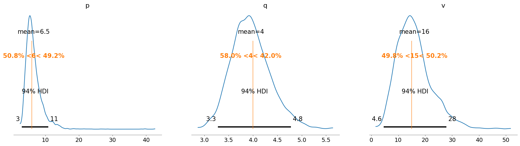
az.plot_posterior(model.fit_result, var_names=["p", "q", "v"], ref_val=[p_true, q_true, v_true]);

expected_spend = model.expected_customer_spend(
    customer_id=idx,
    mean_transaction_value=z_mean,
    frequency=x,
).stack(sample=("draw", "chain"))

Sampling: [nu]

100.00% [4000/4000 00:01<00:00]

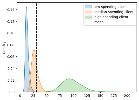
sns.kdeplot(expected_spend.sel(customer_id=selected_idxs[0]), fill=True, label="low spending client")
sns.kdeplot(expected_spend.sel(customer_id=selected_idxs[1]), fill=True, label="median spending client")
sns.kdeplot(expected_spend.sel(customer_id=selected_idxs[2]), fill=True, label="high spending client")
plt.axvline(expected_spend.mean(), color="k", ls="--", label="mean")
plt.legend();

new_spend = model.expected_new_customer_spend().stack(sample=("chain", "draw"))

Sampling: [nu]

100.00% [4000/4000 00:00<00:00]

sns.kdeplot(new_spend.isel(new_customer_id=0), fill=True, label="high spending client")
plt.axvline(new_spend.mean(), color="k", ls="--", label="mean")
plt.legend();

Manual PyMC implementations

We show how the Gamma-Gamma model can be implemented by hand using PyMC. This clarifies how the model can be modified or extended to include more prior information or additional structure.

Gamma-Gamma model conditioned on individual transactions \(z\)

with pm.Model() as m1:
    p = pm.HalfFlat("p")
    q = pm.HalfFlat("q")
    v = pm.HalfFlat("v")
    
    nu = pm.Gamma("nu", q, v, size=N)
    pm.Gamma("z", p, nu[idx], observed=z)

    pm.Deterministic("mean_spend", p / nu)
    
    trace1 = pm.sample(random_seed=rng)

Auto-assigning NUTS sampler...
Initializing NUTS using jitter+adapt_diag...
Multiprocess sampling (4 chains in 4 jobs)
NUTS: [p, q, v, nu]

100.00% [8000/8000 00:20<00:00 Sampling 4 chains, 0 divergences]

Sampling 4 chains for 1_000 tune and 1_000 draw iterations (4_000 + 4_000 draws total) took 21 seconds.

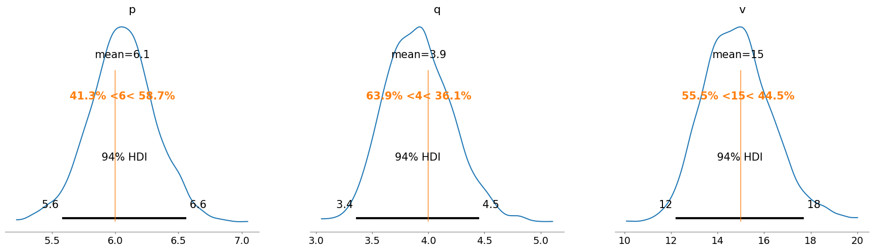
az.summary(trace1, var_names=["p", "q", "v"])

	mean	sd	hdi_3%	hdi_97%	mcse_mean	mcse_sd	ess_bulk	ess_tail	r_hat
p	6.055	0.260	5.578	6.564	0.020	0.014	178.0	382.0	1.02
q	3.914	0.295	3.358	4.453	0.007	0.005	1877.0	1959.0	1.00
v	14.879	1.486	12.194	17.717	0.071	0.050	438.0	1131.0	1.01

az.plot_posterior(trace1, var_names=["p", "q", "v"], ref_val=[p_true, q_true, v_true]);

Gamma-gamma model conditioned on average transactions per user \(\overline{z}\)

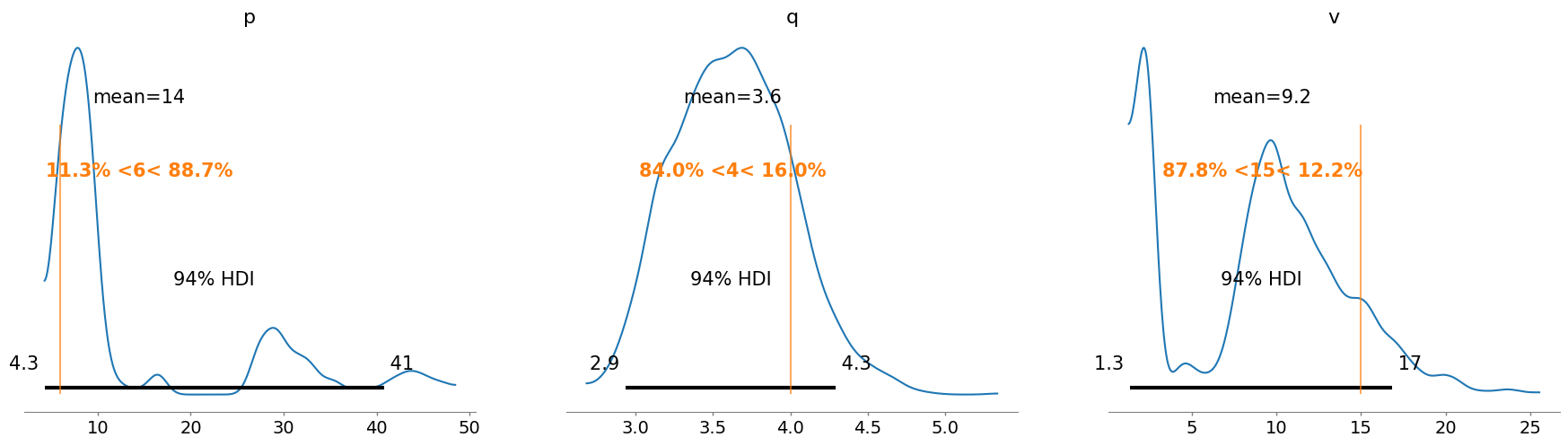
This fails to sample because the model contains “nearly” two independent parameters per observation. For more details check this Discourse topic

with pm.Model() as m2:
    p = pm.HalfFlat("p")
    q = pm.HalfFlat("q")
    v = pm.HalfFlat("v")

    nu = pm.Gamma("nu", q, v, size=N)
    # We use the convolution properties of the gamma distribution to model
    # the mean of multiple transaction using the parameters of individual
    # transactions
    pm.Gamma("z_mean", p*x, nu*x, observed=z_mean)
    
    trace2 = pm.sample(random_seed=rng)

Auto-assigning NUTS sampler...
Initializing NUTS using jitter+adapt_diag...
Multiprocess sampling (4 chains in 4 jobs)
NUTS: [p, q, v, nu]

100.00% [8000/8000 00:26<00:00 Sampling 4 chains, 0 divergences]

Sampling 4 chains for 1_000 tune and 1_000 draw iterations (4_000 + 4_000 draws total) took 27 seconds.

az.summary(trace2, var_names=["p", "q", "v"])

	mean	sd	hdi_3%	hdi_97%	mcse_mean	mcse_sd	ess_bulk	ess_tail	r_hat
p	14.454	11.819	4.299	40.762	5.738	4.375	5.0	11.0	2.17
q	3.629	0.376	2.939	4.294	0.129	0.094	8.0	41.0	1.41
v	9.154	5.062	1.340	16.853	2.264	1.705	5.0	11.0	2.09

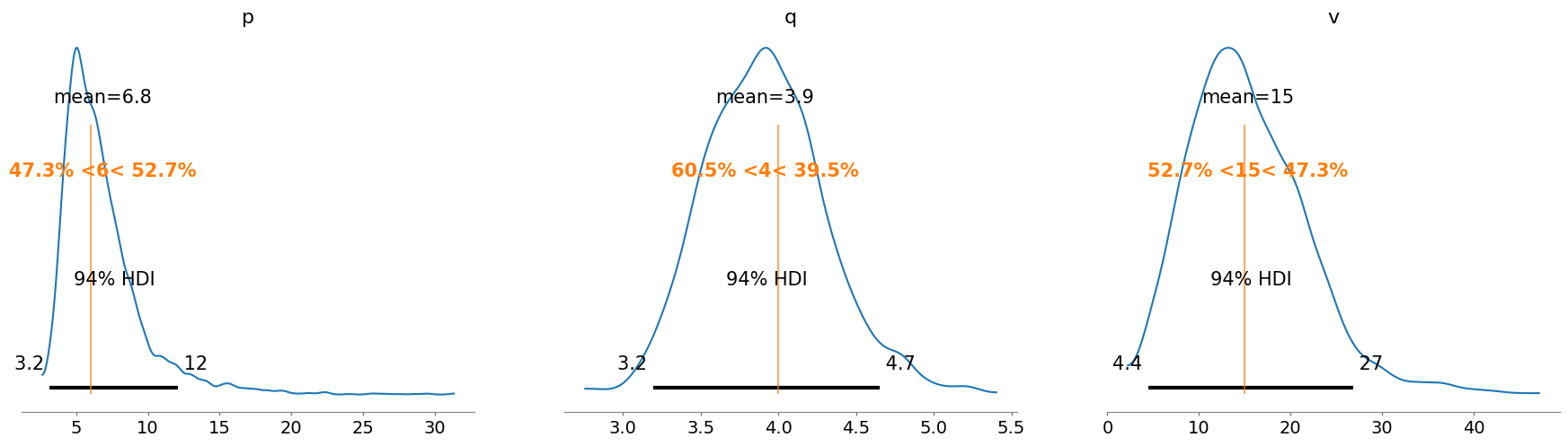
az.plot_posterior(trace2, var_names=["p", "q", "v"], ref_val=[p_true, q_true, v_true]);

Gamma-Gamma model conditioned on average transaction per user with \(\nu\) marginalized

with pm.Model() as m3:
    p = pm.HalfFlat("p")
    q = pm.HalfFlat("q")
    v = pm.HalfFlat("v")

    # Likelihood of z_mean, marginalizing over nu
    likelihood = pm.Potential(
        "likelihood", 
        (
            pt.gammaln(p * x + q)
            - pt.gammaln(p * x)
            - pt.gammaln(q)
            + q * pt.log(v)
            + (p * x - 1) * pt.log(z_mean)
            + (p * x) * pt.log(x)
            - (p * x + q) * pt.log(x * z_mean + v)
        ),
    )

    # Closed form solution posterior individual nu
    nu = pm.Deterministic("nu", pm.Gamma.dist(p * x + q, v + x * z_mean))
    pm.Deterministic("mean_spend", p / nu)
    
    trace3 = pm.sample(random_seed=rng)

Auto-assigning NUTS sampler...
Initializing NUTS using jitter+adapt_diag...
Multiprocess sampling (4 chains in 4 jobs)
NUTS: [p, q, v]

100.00% [8000/8000 00:32<00:00 Sampling 4 chains, 0 divergences]

Sampling 4 chains for 1_000 tune and 1_000 draw iterations (4_000 + 4_000 draws total) took 33 seconds.

az.summary(trace3, var_names=["p", "q", "v"])

	mean	sd	hdi_3%	hdi_97%	mcse_mean	mcse_sd	ess_bulk	ess_tail	r_hat
p	6.845	2.937	3.153	12.110	0.110	0.080	865.0	812.0	1.0
q	3.915	0.390	3.194	4.654	0.012	0.009	974.0	1118.0	1.0
v	15.375	6.510	4.445	26.879	0.221	0.156	816.0	738.0	1.0

az.plot_posterior(trace3, var_names=["p", "q", "v"], ref_val=[p_true, q_true, v_true]);