

import numpy as np
import pandas as pd

import pymc as pm
import xarray as xr

from pymc_marketing.clv import utils
from pymc_marketing.clv import ParetoNBDModel
from pymc_extras.prior import Prior

from pymc_marketing.clv import utils, plotting
OMP: Info #276: omp_set_nested routine deprecated, please use omp_set_max_active_levels instead.
import pytensor

#set flag to fix open issue
pytensor.config.cxx = '/usr/bin/clang++'
Create a simple dataset for testing:
d = [
    [1, "2015-01-01", 1],
    [1, "2015-02-06", 2],
    [2, "2015-01-01", 2],
    [3, "2015-01-01", 3],
    [3, "2015-01-02", 1],
    [3, "2015-01-05", 5],
    [4, "2015-01-16", 6],
    [4, "2015-02-02", 3],
    [4, "2015-02-05", 3],
    [4, "2015-02-05", 2],
    [5, "2015-01-16", 3],
    [5, "2015-01-17", 1],
    [5, "2015-01-18", 8],
    [6, "2015-02-02", 5],
]
test_data = pd.DataFrame(d, columns=["id", "date", "monetary_value"])
Note customer 4 made two purchases on 2015-02-05.
_find_first_transactions flags the first purchase each customer has made, which must be excluded for modeling. It is called internally by rfm_summary.
utils._find_first_transactions(
    transactions=test_data,
    customer_id_col = "id",
    datetime_col = "date",
    #monetary_value_col = "monetary_value",
    #datetime_format = "%Y%m%d",
).reindex()
| id | date | first | |
|---|---|---|---|
| 0 | 1 | 2015-01-01 | True |
| 1 | 1 | 2015-02-06 | False |
| 2 | 2 | 2015-01-01 | True |
| 3 | 3 | 2015-01-01 | True |
| 4 | 3 | 2015-01-02 | False |
| 5 | 3 | 2015-01-05 | False |
| 6 | 4 | 2015-01-16 | True |
| 7 | 4 | 2015-02-02 | False |
| 8 | 4 | 2015-02-05 | False |
| 10 | 5 | 2015-01-16 | True |
| 11 | 5 | 2015-01-17 | False |
| 12 | 5 | 2015-01-18 | False |
| 13 | 6 | 2015-02-02 | True |
Notice how 9 is missing from the dataframe index. Multiple transactions in the same time period are treated as a single purchase, so the indices for those additional transactions are skipped.
rfm_summary is the primary data preprocessing step for CLV modeling in the continuous, non-contractual domain:
rfm_df = utils.rfm_summary(
    test_data,
    customer_id_col = "id",
    datetime_col = "date",
    monetary_value_col = "monetary_value",
    observation_period_end = "2015-02-06",
    datetime_format = "%Y-%m-%d",
    time_unit = "W",
    include_first_transaction=True,
)

rfm_df.head()
| customer_id | frequency | recency | monetary_value | |
|---|---|---|---|---|
| 0 | 1 | 2.0 | 0.0 | 1.5 |
| 1 | 2 | 1.0 | 5.0 | 2.0 |
| 2 | 3 | 2.0 | 4.0 | 4.5 |
| 3 | 4 | 2.0 | 0.0 | 7.0 |
| 4 | 5 | 1.0 | 3.0 | 12.0 |
For MAP fits and covariate models, rfm_train_test_split can be used to evaluate models on unseen data. It is also useful for identifying the impact of a time-based event like a marketing campaign.
train_test = utils.rfm_train_test_split(
    test_data,
    customer_id_col = "id",
    datetime_col = "date",
    train_period_end = "2015-02-01",
    monetary_value_col = "monetary_value",
)

train_test.head()
| customer_id | frequency | recency | T | monetary_value | test_frequency | test_monetary_value | test_T | |
|---|---|---|---|---|---|---|---|---|
| 0 | 1 | 0.0 | 0.0 | 31.0 | 0.0 | 1.0 | 2.0 | 5.0 |
| 1 | 2 | 0.0 | 0.0 | 31.0 | 0.0 | 0.0 | 0.0 | 5.0 |
| 2 | 3 | 2.0 | 4.0 | 31.0 | 3.0 | 0.0 | 0.0 | 5.0 |
| 3 | 4 | 0.0 | 0.0 | 16.0 | 0.0 | 2.0 | 4.0 | 5.0 |
| 4 | 5 | 2.0 | 2.0 | 16.0 | 4.5 | 0.0 | 0.0 | 5.0 |
rfm_segments will assign customer to segments based on their recency, frequency, and monetary value. It uses a quartile-based RFM score approach that is very computationally efficient, but defining custom segments is a rather subjective exercise. The returned dataframe also cannot be used for modeling because it does not zero out the initial transactions.
segments = utils.rfm_segments(
    test_data,
    customer_id_col = "id",
    datetime_col = "date",
    monetary_value_col = "monetary_value",
    observation_period_end = "2015-02-06",
    datetime_format = "%Y-%m-%d",
    time_unit = "W",
)
/Users/coltallen/Projects/pymc-marketing/pymc_marketing/clv/utils.py:702: UserWarning: RFM score will not exceed 2 for f_quartile. Specify a custom segment_config
  warnings.warn(
Plotting#
expected_cumulative_transactions and all other plotting functions require a fitted model. Test with both MAP and full posteriors:
url_cdnow = "https://raw.githubusercontent.com/pymc-labs/pymc-marketing/main/data/cdnow_transactions.csv"
raw_trans = pd.read_csv(url_cdnow)

rfm_data = utils.rfm_summary(
    raw_trans,
    customer_id_col = "id",
    datetime_col = "date",
    datetime_format = "%Y%m%d",
    time_unit = "W",
    observation_period_end = "19970930",
    #time_scaler = 7,
)

rfm_train_test = utils.rfm_train_test_split(
    raw_trans,
    customer_id_col = "id",
    datetime_col = "date",
    train_period_end = "19970701",
    datetime_format = "%Y%m%d",
    time_unit = "W",
    test_period_end = "19970930",
)

t=rfm_data["T"].max().astype(int)
t_start_eval = rfm_train_test["T"].max()

pnbd_split = ParetoNBDModel(data=rfm_data)
pnbd_split.fit()
-
<xarray.Dataset> Size: 48B Dimensions: (chain: 1, draw: 1) Coordinates: * chain (chain) int64 8B 0 * draw (draw) int64 8B 0 Data variables: alpha (chain, draw) float64 8B 14.46 beta (chain, draw) float64 8B 10.48 r (chain, draw) float64 8B 0.6338 s (chain, draw) float64 8B 0.4882 Attributes: created_at: 2025-09-17T17:06:17.639985+00:00 arviz_version: 0.22.0 inference_library: pymc inference_library_version: 5.25.1 -
<xarray.Dataset> Size: 57kB Dimensions: (customer_id: 2357, obs_var: 2) Coordinates: * customer_id (customer_id) int64 19kB 1 2 3 4 ... 2354 2355 2356 2357 * obs_var (obs_var) <U9 72B 'recency' 'frequency' Data variables: recency_frequency (customer_id, obs_var) float64 38kB 30.0 2.0 ... 0.0 0.0 Attributes: created_at: 2025-09-17T17:06:17.644276+00:00 arviz_version: 0.22.0 inference_library: pymc inference_library_version: 5.25.1 -
<xarray.Dataset> Size: 94kB
Dimensions:      (index: 2357)
Coordinates:
  * index        (index) int64 19kB 0 1 2 3 4 5 ... 2352 2353 2354 2355 2356
Data variables:
    customer_id  (index) int64 19kB 1 2 3 4 5 6 ... 2353 2354 2355 2356 2357
    frequency    (index) float64 19kB 2.0 1.0 0.0 0.0 0.0 ... 5.0 0.0 4.0 0.0
    recency      (index) float64 19kB 30.0 2.0 0.0 0.0 0.0 ... 24.0 0.0 26.0 0.0
    T            (index) float64 19kB 39.0 39.0 39.0 39.0 ... 27.0 27.0 27.0
Expected Cumulative Purchases#
df_cum = utils._expected_cumulative_transactions(
    model=pnbd_split,
    transactions=raw_trans,
    customer_id_col="id",
    datetime_col="date",
    t=t,
    datetime_format="%Y%m%d",
    time_unit="W",
    set_index_date=True,
)

df_cum.head()
| actual | predicted | |
|---|---|---|
| 1996-12-30/1997-01-05 | 0 | 4.286469 |
| 1997-01-06/1997-01-12 | 3 | 15.595394 |
| 1997-01-13/1997-01-19 | 17 | 33.947389 |
| 1997-01-20/1997-01-26 | 44 | 59.853467 |
| 1997-01-27/1997-02-02 | 67 | 93.519782 |
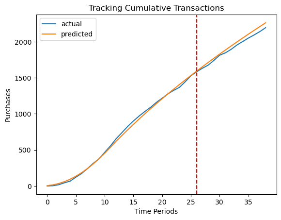
If doing a train/test split, or studying time interventions like marketing campaigns, plot_expected_purchases_over_time can be used for easy visual interpretation.
plotting.plot_expected_purchases_over_time(
    model=pnbd_split,
    purchase_history=raw_trans,
    customer_id_col="id",
    datetime_col="date",
    t=t,
    t_start_eval = t_start_eval,
    datetime_format="%Y%m%d",
    time_unit="W",
    plot_cumulative=True,
)
<Axes: title={'center': 'Tracking Cumulative Transactions'}, xlabel='Time Periods', ylabel='Purchases'>
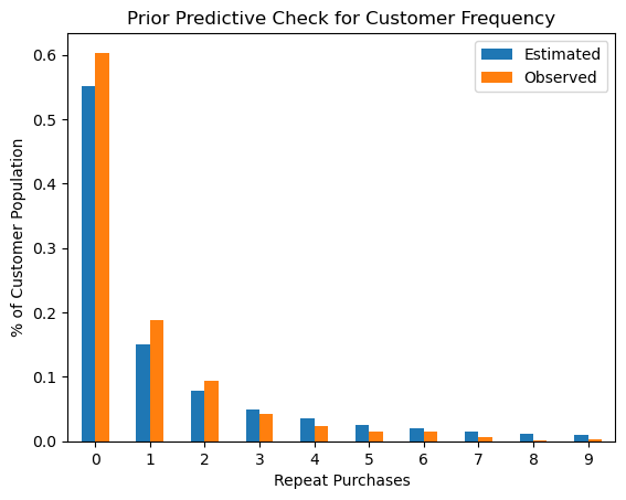
plotting.plot_expected_purchases_ppc(pnbd_split, ppc='prior');
Sampling: [alpha, beta, r, recency_frequency, s]
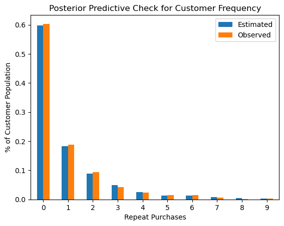
from matplotlib import pyplot as plt

fig = plt.figure()

fig.add_axes(plotting.plot_expected_purchases_ppc(pnbd_split, ppc='posterior'))

fig.savefig("save_test.png");
Sampling: [recency_frequency]
Now fit a model by sampling from the posterior distributions:
pnbd = ParetoNBDModel(data=rfm_data)

pnbd.build_model()
with pnbd.model:
    pnbd.idata = pm.sample(
        step=pm.DEMetropolisZ(),
        tune=2500,
        draws=3000,
        idata_kwargs={"log_likelihood": True},
    )
pnbd.fit_summary()
| mean | sd | hdi_3% | hdi_97% | mcse_mean | mcse_sd | ess_bulk | ess_tail | r_hat | |
|---|---|---|---|---|---|---|---|---|---|
| alpha | 14.596 | 1.114 | 12.445 | 16.640 | 0.042 | 0.030 | 712.0 | 1280.0 | 1.01 |
| beta | 12.043 | 3.800 | 5.029 | 18.742 | 0.127 | 0.090 | 862.0 | 1294.0 | 1.00 |
| r | 0.640 | 0.054 | 0.545 | 0.742 | 0.002 | 0.001 | 894.0 | 1132.0 | 1.01 |
| s | 0.529 | 0.105 | 0.340 | 0.729 | 0.004 | 0.003 | 842.0 | 1553.0 | 1.01 |
# thin_fit_result is not supported with external sampler fits in `ParetoNBDModel`!
#pnbd.idata = pnbd.thin_fit_result(keep_every=3)

pnbd.idata = pnbd.idata.isel(draw=slice(None, None, 3)).copy()
pnbd.idata
-
<xarray.Dataset> Size: 136kB Dimensions: (chain: 4, draw: 1000) Coordinates: * chain (chain) int64 32B 0 1 2 3 * draw (draw) int64 8kB 0 3 6 9 12 15 18 ... 2982 2985 2988 2991 2994 2997 Data variables: alpha (chain, draw) float64 32kB 14.46 12.74 12.74 ... 13.8 13.8 13.8 beta (chain, draw) float64 32kB 10.87 14.3 14.3 ... 13.58 13.58 13.58 r (chain, draw) float64 32kB 0.6681 0.56 0.56 ... 0.5876 0.5876 s (chain, draw) float64 32kB 0.5164 0.5783 0.5783 ... 0.5571 0.5571 Attributes: created_at: 2024-11-23T22:39:12.899029+00:00 arviz_version: 0.18.0 inference_library: pymc inference_library_version: 5.15.1 sampling_time: 6.328435897827148 tuning_steps: 2500 -
<xarray.Dataset> Size: 75MB Dimensions: (chain: 4, draw: 1000, customer_id: 2357) Coordinates: * chain (chain) int64 32B 0 1 2 3 * draw (draw) int64 8kB 0 3 6 9 12 ... 2985 2988 2991 2994 2997 * customer_id (customer_id) int64 19kB 1 2 3 4 ... 2354 2355 2356 2357 Data variables: recency_frequency (chain, draw, customer_id) float64 75MB -9.378 ... -0.... Attributes: created_at: 2024-11-23T22:39:18.592759+00:00 arviz_version: 0.18.0 inference_library: pymc inference_library_version: 5.15.1 -
<xarray.Dataset> Size: 108kB Dimensions: (chain: 4, draw: 1000) Coordinates: * chain (chain) int64 32B 0 1 2 3 * draw (draw) int64 8kB 0 3 6 9 12 15 ... 2982 2985 2988 2991 2994 2997 Data variables: accept (chain, draw) float64 32kB 8.341 0.01704 ... 0.03161 0.627 accepted (chain, draw) bool 4kB True False False ... False False False lambda (chain, draw) float64 32kB 0.8415 0.8415 0.8415 ... 0.8415 0.8415 scaling (chain, draw) float64 32kB 0.0002288 0.0002288 ... 0.001 0.001 Attributes: created_at: 2024-11-23T22:39:12.901456+00:00 arviz_version: 0.18.0 inference_library: pymc inference_library_version: 5.15.1 sampling_time: 6.328435897827148 tuning_steps: 2500 -
<xarray.Dataset> Size: 57kB
Dimensions:            (customer_id: 2357, obs_var: 2)
Coordinates:
  * customer_id        (customer_id) int64 19kB 1 2 3 4 ... 2354 2355 2356 2357
  * obs_var            (obs_var) <U9 72B 'recency' 'frequency'
Data variables:
    recency_frequency  (customer_id, obs_var) float64 38kB 30.0 2.0 ... 0.0 0.0
Attributes:
    created_at:                 2024-11-23T22:39:12.902959+00:00
    arviz_version:              0.18.0
    inference_library:          pymc
    inference_library_version:  5.15.1
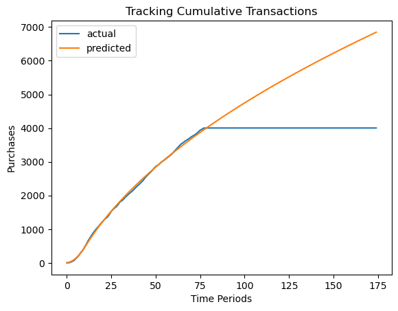
plotting.plot_expected_purchases(
    model=pnbd,
    purchase_history=raw_trans,
    customer_id_col="id",
    datetime_col="date",
    t=25*7,
    datetime_format="%Y%m%d",
    time_unit="W",
    plot_cumulative=True,
)
<Axes: title={'center': 'Tracking Cumulative Transactions'}, xlabel='Time Periods', ylabel='Purchases'>
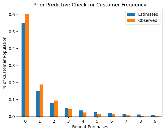
plotting.plot_expected_purchases_ppc(pnbd, ppc='prior');
Sampling: [alpha, beta, r, recency_frequency, s]
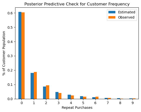
plotting.plot_expected_purchases_ppc(pnbd, ppc='posterior');
Sampling: [recency_frequency]
Adding HDIs to plot_purchase_pmf requires value counts to be grouped coordinate-wise across a dimension like draws, which may not be supported in xarray. arviz.hdi can then be applied across all value counts for interval estimation.
# keep n_samples=1
pnbd.distribution_new_customer_recency_frequency(
        random_seed=45,
        n_samples=1,
    ).sel(obs_var="frequency")
Sampling: [recency_frequency]
<xarray.DataArray 'recency_frequency' (chain: 4, draw: 1000, customer_id: 2357)> Size: 75MB
array([[[ 2.,  0.,  0., ...,  7.,  1.,  1.],
        [ 0.,  0.,  0., ...,  0.,  0.,  0.],
        [ 0.,  2.,  0., ...,  0.,  4.,  0.],
        ...,
        [ 8.,  2., 10., ...,  7.,  0.,  1.],
        [ 1.,  0.,  0., ...,  0.,  0.,  0.],
        [ 0.,  0.,  1., ...,  2.,  6.,  0.]],

       [[ 1.,  3.,  0., ...,  1.,  2.,  0.],
        [ 0.,  0.,  0., ...,  0.,  1.,  0.],
        [ 0.,  3.,  0., ...,  0.,  2.,  4.],
        ...,
        [ 2.,  0.,  0., ...,  0.,  2.,  0.],
        [ 0.,  0.,  4., ...,  0.,  1.,  3.],
        [ 0.,  0.,  0., ...,  0.,  0.,  2.]],

       [[ 1.,  0.,  1., ...,  3.,  0.,  0.],
        [ 1.,  1.,  0., ...,  3.,  0.,  0.],
        [ 0.,  1.,  0., ...,  0.,  2.,  0.],
        ...,
        [ 0.,  0.,  0., ...,  0.,  6.,  0.],
        [ 1.,  0.,  0., ...,  0.,  1.,  0.],
        [ 0.,  0.,  0., ...,  0.,  0.,  1.]],

       [[ 1.,  0.,  0., ...,  0.,  0.,  1.],
        [ 3.,  0.,  0., ...,  2.,  0.,  0.],
        [ 4.,  1.,  0., ...,  2.,  5.,  0.],
        ...,
        [ 1.,  0.,  3., ...,  2.,  3.,  0.],
        [ 0.,  0.,  1., ...,  0.,  0.,  0.],
        [ 0.,  0.,  0., ...,  2.,  0.,  0.]]])
Coordinates:
  * chain        (chain) int64 32B 0 1 2 3
  * draw         (draw) int64 8kB 0 3 6 9 12 15 ... 2985 2988 2991 2994 2997
  * customer_id  (customer_id) int64 19kB 1 2 3 4 5 ... 2353 2354 2355 2356 2357
obs_var <U9 36B 'frequency'import pymc as pm
import xarray as xr
# TODO: Add build_model() before a prior predictive check
pnbd.build_model()
with pnbd.model:
prior_idata = pm.sample_prior_predictive(random_seed=45, draws=100)
# obs_var must be obtained from prior_idata in case of an unfit model
obs_freq = prior_idata.observed_data["recency_frequency"].sel(obs_var="frequency")
ppc_freq = prior_idata.prior_predictive["recency_frequency"].sel(obs_var="frequency")#.mean(("chain","draw"))
#ppc_freq = prior_idata.prior_predictive["recency_frequency"].sel(obs_var="frequency").mean(("chain","draw"))#.rename({o
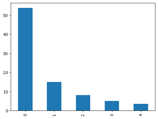
ppc_df = ppc_freq.to_dataframe()['recency_frequency'].value_counts(normalize=True).sort_index() * 100
# Percentages are the only way to compare actual counts to chain*draw simulated counts
# merged_xr.to_dataframe()["recency_frequency"].value_counts(normalize=True) * 100
# merged_xr.to_dataframe()["ppc_mean"].value_counts(normalize=True) * 100
Sampling: [alpha, beta, r, recency_frequency, s]
ppc_df.reset_index()['proportion'].head(5).plot(kind='bar')
<Axes: >
from xarray.groupers import UniqueGrouper

# This will do value counts for entire DataArray
#ppc_freq.groupby(ppc_freq).count()
#ppc_freq.groupby(chain=UniqueGrouper()).count()

#value_counts = xr.DataArray(np.bincount(ppc_freq.values), dims="value")
#np.bincount(ppc_freq.values)
xr.DataArray([1, 2, 2, 3, 3, 3], dims="x")
# but what about individual customers?
# create a value count coordinate
# prior_idata.prior_predictive.coords["value_counts"] = ppc_freq.groupby(ppc_freq).count()["ppc_mean"].values
# ppc_freq = prior_idata.rename_vars({"recency_frequency":"ppc_mean"}).prior_predictive["ppc_mean"]#.sel(obs_var="frequency")#.mean(("chain","draw"))
# ppc_freq
# prior_idata.prior_predictive.groupby(value_counts=UniqueGrouper()).count().sel(obs_var="frequency")
#prior_idata.prior_predictive.groupby("customer_id").count()
#prior_idata#
#
# #ppc_freq.coords["grouped_customer"]
#ppc_freq.groupby(draw=UniqueGrouper()).count()
<xarray.DataArray (x: 6)> Size: 48B
array([1, 2, 2, 3, 3, 3])
Dimensions without coordinates: x
from arviz.stats import hdi

calc_hdi = hdi(
    ary=prior_idata,
    hdi_prob=.9, #param
    group='prior_predictive', #posterior
).sel(obs_var='frequency')

hdi_lo = calc_hdi.sel(hdi='lower').to_array().squeeze()
hdi_hi = calc_hdi.sel(hdi='higher').to_array().squeeze()

# TODO: Join back to ppc_freq & obs var
hdi_hi
<xarray.DataArray (customer_id: 2357)> Size: 19kB
array([6., 5., 9., ..., 6., 6., 6.])
Coordinates:
  * customer_id  (customer_id) int64 19kB 1 2 3 4 5 ... 2353 2354 2355 2356 2357
    obs_var      <U9 36B 'frequency'
    hdi          <U6 24B 'higher'
    variable     <U17 68B 'recency_frequency'