Model Configuration#
This goes over the model configuration
Setup#
import arviz as az
import matplotlib.pyplot as plt
import numpy as np
import pandas as pd
import pymc as pm

from pymc_marketing.model_config import ModelConfigError, parse_model_config
from pymc_marketing.prior import Prior

az.style.use("arviz-darkgrid")
plt.rcParams["figure.figsize"] = [12, 7]
plt.rcParams["figure.dpi"] = 100
seed = sum(map(ord, "Create priors to reflect your marketing beliefs"))
rng = np.random.default_rng(seed)
Prior Distributions#
The Prior class is our way to expression distributions and relationships between them.
Basic Usage#
Every prior will need a distribution name that comes from PyMC. View the full list in the documentation here.
scalar_distribution = Prior("Normal")
scalar_distribution
Prior("Normal")
If not, then an exception will be raised.
try:
    Prior("UnknownDistribution")
except Exception as e:
    print(e)
PyMC doesn't have a distribution of name 'UnknownDistribution'
Specific parameters can be passed as keyword arguments but are not required if the PyMC distribution has defaults.
scalar_distribution = Prior("Normal", mu=0, sigma=3.5)
scalar_distribution
Prior("Normal", mu=0, sigma=3.5)
There will be a check at initialization against the PyMC distribution.
try:
    Prior("Normal", mu=0, b=1)
except Exception as e:
    print(e)
Parameters {'b', 'mu'} are not a subset of the pymc distribution parameters {'mu', 'tau', 'sigma'}
However, there are some limitations to that. Take this invalid parameterization below:
invalid_distribution = Prior("Normal", mu=1, sigma=1, tau=2)
The create_variable method is used to make variables from this distribution and it isn’t until then that there is an error.
with pm.Model():
    try:
        invalid_distribution.create_variable("mu")
    except Exception as e:
        print(e)
Can't pass both tau and sigma
This goes for incorrect values as well!
invalid_distribution = Prior("Normal", mu=1, sigma=-1)
invalid_distribution
Prior("Normal", mu=1, sigma=-1)
The dims parameter are used to express the dimensions of the distribution. This variable is not part of a model so the values are not reflected with the distribution itself.
vector_distribution = Prior("Normal", dims="channel")
vector_distribution
Prior("Normal", dims="channel")
If there are dimensions, then the coords need to exist in the larger model. But they exist separately and can defined in advance.
Tip
Each Prior instance is just instructions to create a variable, so they can be used multiple times!
coords = {"channel": ["C1", "C2"]}
with pm.Model(coords=coords) as model:
    alpha = vector_distribution.create_variable("alpha")
    beta = vector_distribution.create_variable("beta")

pm.model_to_graphviz(model)

If the coords were not specified then this would cause a PyMC error.
with pm.Model() as model:
    try:
        vector_distribution.create_variable("var")
    except Exception as e:
        print(e)
"Dimensions {'channel'} are unknown to the model and cannot be used to specify a `shape`."
The variables can get arbitrarily large as well by providing additional dims in a tuple.
matrix_distribution = Prior("Normal", dims=("channel", "geo"))
matrix_distribution
Prior("Normal", dims=("channel", "geo"))
tensor_distribution = Prior("Normal", dims=("channel", "geo", "store"))
tensor_distribution
Prior("Normal", dims=("channel", "geo", "store"))
Hierarchical Variables#
Hierarchical variables can be defined by using distributions as the parameters of another distribution. The parent distributions will usually have a larger dimensionality than each of the parameters.
hierarchical_variable = Prior(
    "Normal",
    mu=Prior("Normal"),
    sigma=Prior("HalfNormal"),
    dims="channel",
)
We can use the to_graph method to create visualize the variable with dummy coordinates.
Note
No need to worry about variable naming! The child parameters will all be automatically named based on the parent.
hierarchical_variable.to_graph()

Warning
The validity of the parameter values will not be checked.
There can be negative sigma parameter in a Normal distribution whether that comes from value or another distribution!
Prior("Normal", mu=1, sigma=-1)
Prior("Normal", mu=1, sigma=-1)
Prior("Normal", sigma=Prior("Normal"))
Prior("Normal", sigma=Prior("Normal"))
Tip
Model reparamterizations can help with model convergence depending on the model posterior!
For Normal distribution, the common non-centered parameterization is supported with the centered flag.
non_centered_hierarchical_variable = Prior(
    "Normal",
    mu=Prior("Normal"),
    sigma=Prior("HalfNormal"),
    dims="channel",
    # Flag for non-centered
    centered=False,
)
non_centered_hierarchical_variable.to_graph()

Other distributions can be hierarchical as well. Just use distributions for parameters of a parent distribution. For instance, the Beta distribution has two positive parameters, alpha and beta which can be reflect as HalfNormal distributions.
zero_to_one_variable = Prior(
    "Beta",
    alpha=Prior("HalfNormal"),
    beta=Prior("HalfNormal"),
    dims="channel",
)
zero_to_one_variable.to_graph()

Transformations#
The transform variable can be used for any of the distributions to change its domain.
These transformations will be taken from pytensor.tensor or pm.math in that order.
Below is a non-centered hierarchical Normal distribution that is put through a sigmoid function in order to change the domain to (0, 1).
hierarchical_zero_to_one_distribution = Prior(
    "Normal",
    mu=Prior("Normal"),
    sigma=Prior("HalfNormal"),
    dims="channel",
    centered=False,
    transform="sigmoid",
)
hierarchical_zero_to_one_distribution.to_graph()

Prior Visualization#
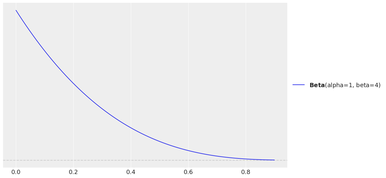
For scalar distributions, make use of the preliz attribute of the model in order to visualize.
Tip
Defaults for the parameters will have to be provided or there will be an error.
beta_distribution = Prior("Beta", alpha=1, beta=4)

beta_distribution.preliz.plot_pdf();
Tip
Using the constrain method can help hone in on a prior. It is a wrapper around the ever-so-helpful find_constrained_prior function. The init_guess is taken to be the parameters of the instance distribution.
constrained_distribution = Prior("Normal", mu=5, sigma=1).constrain(lower=4, upper=6)
constrained_distribution
Prior("Normal", mu=5.000013661179942, sigma=0.5102135210258302)
For more complicated distributions, consider using the sample_prior method in order to access the prior.
Note
Any coordinates will have to be passed like in pm.Model.
complicated_distribution = Prior(
    "Normal",
    mu=Prior("Normal", sigma=1),
    sigma=Prior("Normal", mu=-1, sigma=0.15, transform="exp"),
    centered=False,
    dims="channel",
    transform="sigmoid",
)

coords = {
    "channel": ["C1", "C2"],
}
prior = complicated_distribution.sample_prior(coords=coords, random_seed=rng)
prior
Sampling: [var_raw_mu, var_raw_offset, var_raw_sigma_raw]
<xarray.Dataset> Size: 40kB
Dimensions:            (chain: 1, draw: 500, channel: 2)
Coordinates:
  * chain              (chain) int64 8B 0
  * draw               (draw) int64 4kB 0 1 2 3 4 5 ... 494 495 496 497 498 499
  * channel            (channel) <U2 16B 'C1' 'C2'
Data variables:
    var_raw_offset     (chain, draw, channel) float64 8kB -0.4456 ... 0.2922
    var_raw_sigma      (chain, draw) float64 4kB 0.3459 0.4046 ... 0.436 0.3669
    var_raw_sigma_raw  (chain, draw) float64 4kB -1.062 -0.905 ... -1.003
    var                (chain, draw, channel) float64 8kB 0.336 ... 0.1463
    var_raw            (chain, draw, channel) float64 8kB -0.6811 ... -1.764
    var_raw_mu         (chain, draw) float64 4kB -0.527 1.038 ... -1.258 -1.871
Attributes:
    created_at:                 2024-07-01T15:12:27.403724
    arviz_version:              0.17.1
    inference_library:          pymc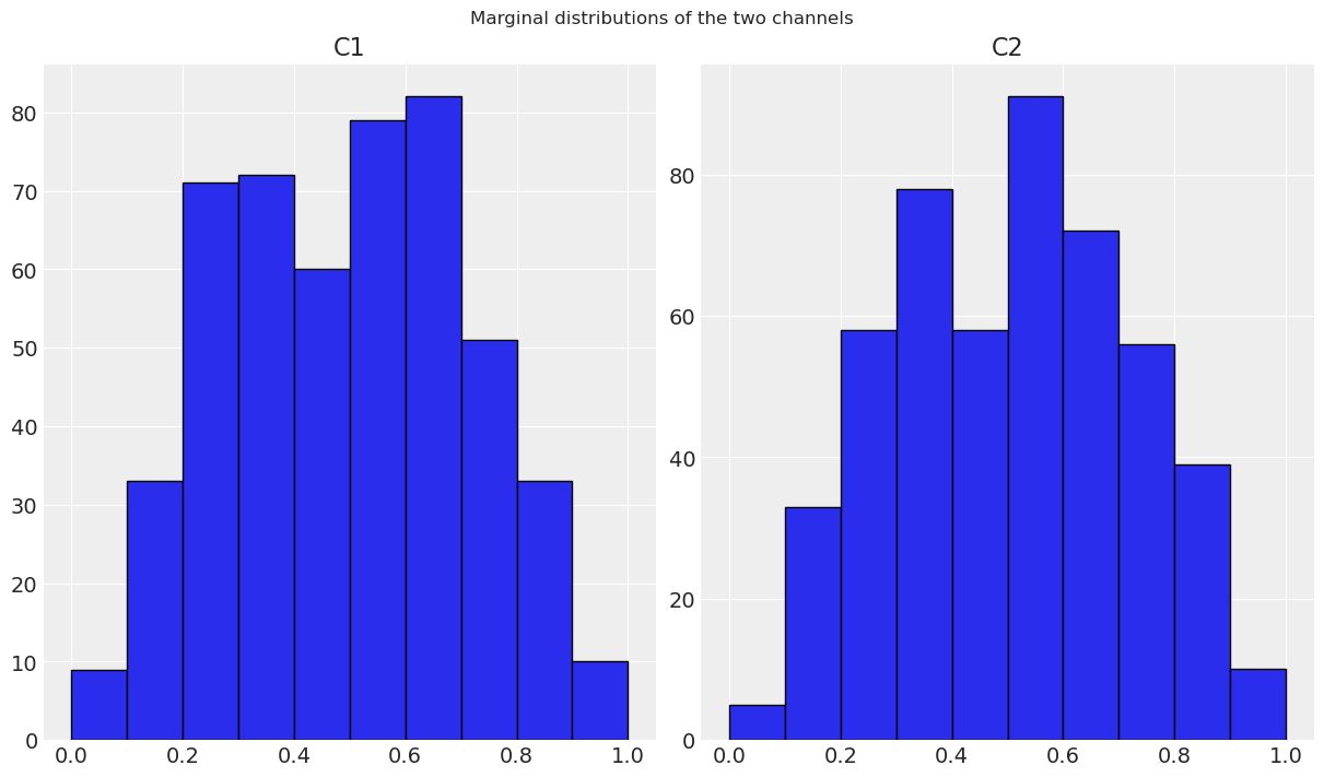
inference_library_version: 5.14.0The prior variables can be visualized in whatever way works best. Here is a histogram of the variables to see the marginal distributions.
bins = np.arange(0, 1.1, 0.1)
prior["var"].to_series().unstack().hist(bins=bins, edgecolor="black")
plt.gcf().suptitle("Marginal distributions of the two channels");
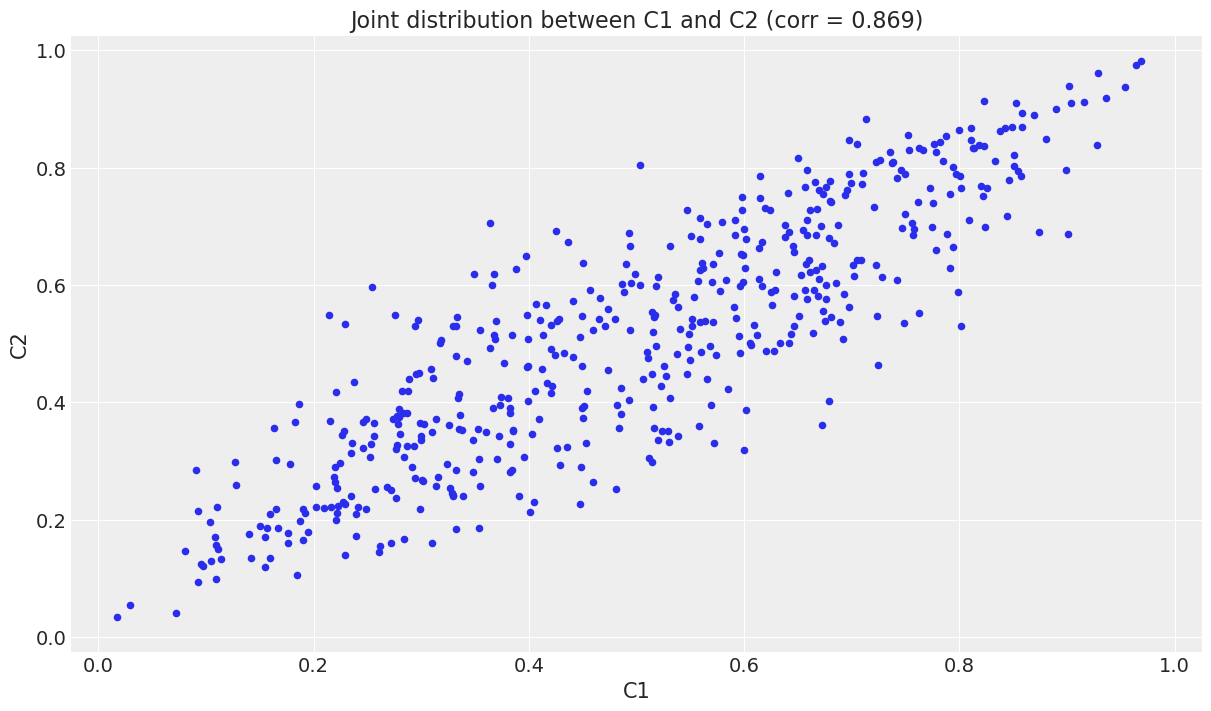
Use any workflow to make sense of the prior distribution! For instance, the joint distribution which shows these two channels are correlated due to the hierarchical generation.
def plot_correlation(df: pd.DataFrame, x: str = "C1", y: str = "C2") -> plt.Axes:
    corr = df.loc[:, [x, y]].corr().iloc[0, 1]
    title = f"Joint distribution between {x} and {y} ({corr = :.3f})"
    return df.plot.scatter(x=x, y=y, title=title)


ax = prior["var"].to_series().unstack().pipe(plot_correlation)
padding = 0.025
bounds = (0 - padding, 1 + padding)
ax.set(xlim=bounds, ylim=bounds);
Automatic Broadcasting#
The broadcasting of the dims will be handled automatically.
For instance, the mu of the variable needs to be transposed in order to work with (“channel”, “geo”) dims.
With all this functionality, we can see that the prior distributions can become quite expressive!
def create_2d_variable(mu_dims, sigma_dims) -> Prior:
    mu = Prior(
        "Normal",
        mu=Prior("Normal"),
        sigma=Prior("HalfNormal"),
        dims=mu_dims,
    )
    sigma = Prior(
        "Normal",
        mu=Prior("Normal"),
        sigma=Prior("HalfNormal"),
        centered=False,
        dims=sigma_dims,
        transform="exp",
    )
    return Prior(
        "Normal",
        mu=mu,
        sigma=sigma,
        dims=("channel", "geo"),
    )


variable_2d = create_2d_variable(mu_dims="channel", sigma_dims="geo")
variable_2d.to_graph()

And the user can spend more time thinking about just the assumptions of the variables rather than logic to ensure the dimensions work.
different_assumptions_2d = create_2d_variable(mu_dims="channel", sigma_dims="channel")

different_assumptions_2d.to_graph()

Serialization#
The to_json and from_json methods can be helpful for storage of the distributions.
variable_2d_dict = variable_2d.to_json()
variable_2d_dict
{'dist': 'Normal',
 'kwargs': {'mu': {'dist': 'Normal',
   'kwargs': {'mu': {'dist': 'Normal'}, 'sigma': {'dist': 'HalfNormal'}},
   'dims': ('channel',)},
  'sigma': {'dist': 'Normal',
   'kwargs': {'mu': {'dist': 'Normal'}, 'sigma': {'dist': 'HalfNormal'}},
   'centered': False,
   'dims': ('geo',),
   'transform': 'exp'}},
 'dims': ('channel', 'geo')}
Prior.from_json(variable_2d_dict).to_graph()
Use in PyMC-Marketing#
Distributions will be expressed in this manner throughout the package including but not limited to:
MMM components
Backwards compatibility#
The from_json method will create a Prior instance from the previous format.
For instance, take this previous configuration:
old_model_config = {
    "alpha": {
        "dist": "Normal",
        "kwargs": {
            "mu": 0,
            "sigma": 1,
        },
    },
    "beta": {
        "dist": "Laplace",
        "kwargs": {
            "mu": 1,
            "b": 0.5,
        },
    },
}
This can be parsed with the Prior.from_json constructor for each key. Much more consise too!
new_model_config = {
    name: Prior.from_json(key) for name, key in old_model_config.items()
}

new_model_config
{'alpha': Prior("Normal", mu=0, sigma=1),
 'beta': Prior("Laplace", mu=1, b=0.5)}
new_model_config["alpha"].to_json()
{'dist': 'Normal', 'kwargs': {'mu': 0, 'sigma': 1}}
The parse_model_config function will do just this and is used internally. It also provides some deprecation warnings.
parse_model_config(old_model_config)
{'alpha': Prior("Normal", mu=0, sigma=1),
 'beta': Prior("Laplace", mu=1, b=0.5)}
As well as the ability to catch some errors while parsing.
invalid_model_config = {
    "alpha": {
        "dist": "InvalidDistribution",
    },
    "beta": {
        "dist": "Normal",
        "kwargs": {"mu": "one", "sigma": "two"},
    },
    "gamma": {
        "dist": "HalfNormal",
        "kwargs": {"mu": 1},
    },
}

try:
    parse_model_config(invalid_model_config)
except ModelConfigError as e:
    print(e)
3 errors occurred while parsing model configuration. Errors: Parameter alpha: PyMC doesn't have a distribution of name 'InvalidDistribution', Parameter beta: Parameters must be one of the following types: (int, float, np.array, Prior, pt.TensorVariable). Incorrect parameters: {'mu': <class 'str'>, 'sigma': <class 'str'>}, Parameter gamma: Parameters {'mu'} are not a subset of the pymc distribution parameters {'sigma', 'tau'}
%load_ext watermark
%watermark -n -u -v -iv -w -p pytensor
Last updated: Mon Jul 01 2024

Python implementation: CPython
Python version       : 3.10.13
IPython version      : 8.22.2

pytensor: 2.20.0

arviz     : 0.17.1
pymc      : 5.14.0
numpy     : 1.26.4
matplotlib: 3.8.3
pandas    : 2.2.1

Watermark: 2.4.3