MMM Example Notebook#

In this notebook we work out a simulated example to showcase the media mix Model (MMM) API from pymc-marketing. This package provides a pymc implementation of the MMM presented in the paper Jin, Yuxue, et al. “Bayesian methods for media mix modeling with carryover and shape effects.” (2017). We work with synthetic data as we want to do parameter recovery to better understand the model assumptions. That is, we explicitly set values for our adstock and saturation parameters (see model specification below) and recover them back from the model. The data generation process is as an adaptation of the blog post “Media Effect Estimation with PyMC: Adstock, Saturation & Diminishing Returns” by Juan Orduz.

Business Problem#

Before jumping into the data, let’s first define the business problem we are trying to solve. We are a marketing agency and we want to optimize the marketing budget of a client. We have access to the following data:

Sales data: weekly sales of the client.
Media spend data: weekly spend on different media channels (e.g. TV, radio, online, etc.). In ths example we consider 2 media channels: \(x_{1}\) and \(x_{2}\).
Domain knowledge:
- We know that there has a been an positive sales trend which we believe comes from a strong economic growth.
- We also know that there is a yearly seasonality effect.
- In addition, we were informed about two outliers in the data during the weeks 2019-05-13 and 2021-09-14.

What do we mean by optimize the marketing budget? We want to find the optimal media mix that maximizes sales. In order to do so, we need to understand the mechanism in which the media spend for each channel affects sales. In other words, we need to understand the media contribution. The main challenge is that the direct cost signal does not translate into a linear contribution. For example, a \(10\%\) increase in channel \(x_{1}\) spend does not necessarily translate into a \(10\%\) increase in sales. This can be explained by two phenomena

On the one hand side, there is a carry-over effect. That is, the effect of spend on sales is not instantaneous but accumulates over time.
In addition, there is a saturation effect. That is, the effect of spend on sales is not linear but saturates at some point.

In this example we will illustrate how we can use pymc-marketing to model these effects.

In the next section we describe a general framework for modeling media effects.

Model Specification#

In pymc-marketing we provide an API for a Bayesian media mix model (MMM) specification following Jin, Yuxue, et al. “Bayesian methods for media mix modeling with carryover and shape effects.” (2017).. Concretely, given a time series target variable \(y_{t}\) (e.g. sales or conversions), media variables \(x_{m, t}\) (e.g. impressions, clicks or costs) and a set of control covariates \(z_{c, t}\) (e.g. holidays, special events) we consider a linear model of the form

\[ y_{t} = \alpha + \sum_{m=1}^{M}\beta_{m}f(x_{m, t}) + \sum_{c=1}^{C}\gamma_{c}z_{c, t} + \varepsilon_{t}, \]

where \(\alpha\) is the intercept, \(f\) is a media transformation function and \(\varepsilon_{t}\) is the error therm which we assume is normally distributed. The function \(f\) encodes the contribution of media on the target variable. Typically we consider two types of transformation: adstock (carry-over) and saturation effects.

References:#

Part I: Data Generation Process#

In Part I of this notebook we focus on the data generating process. That is, we want to construct the target variable \(y_{t}\) (sales) by adding each of the components described in the Business Problem section.

Prepare Notebook#

import warnings

import arviz as az
import matplotlib.pyplot as plt
import numpy as np
import pandas as pd
import pymc as pm
import seaborn as sns

from pymc_marketing.mmm.delayed_saturated_mmm import DelayedSaturatedMMM
from pymc_marketing.mmm.transformers import geometric_adstock, logistic_saturation

warnings.filterwarnings("ignore")

az.style.use("arviz-darkgrid")
plt.rcParams["figure.figsize"] = [12, 7]
plt.rcParams["figure.dpi"] = 100

%load_ext autoreload
%autoreload 2
%config InlineBackend.figure_format = "retina"

Generate Data#

1. Date Range#

First we set a time range for our data. We consider a bit more than 2 years of data at weekly granularity.

seed: int = sum(map(ord, "mmm"))
rng: np.random.Generator = np.random.default_rng(seed=seed)

# date range
min_date = pd.to_datetime("2018-04-01")
max_date = pd.to_datetime("2021-09-01")

df = pd.DataFrame(
    data={"date_week": pd.date_range(start=min_date, end=max_date, freq="W-MON")}
).assign(
    year=lambda x: x["date_week"].dt.year,
    month=lambda x: x["date_week"].dt.month,
    dayofyear=lambda x: x["date_week"].dt.dayofyear,
)

n = df.shape[0]
print(f"Number of observations: {n}")

Number of observations: 179

2. Media Costs Data#

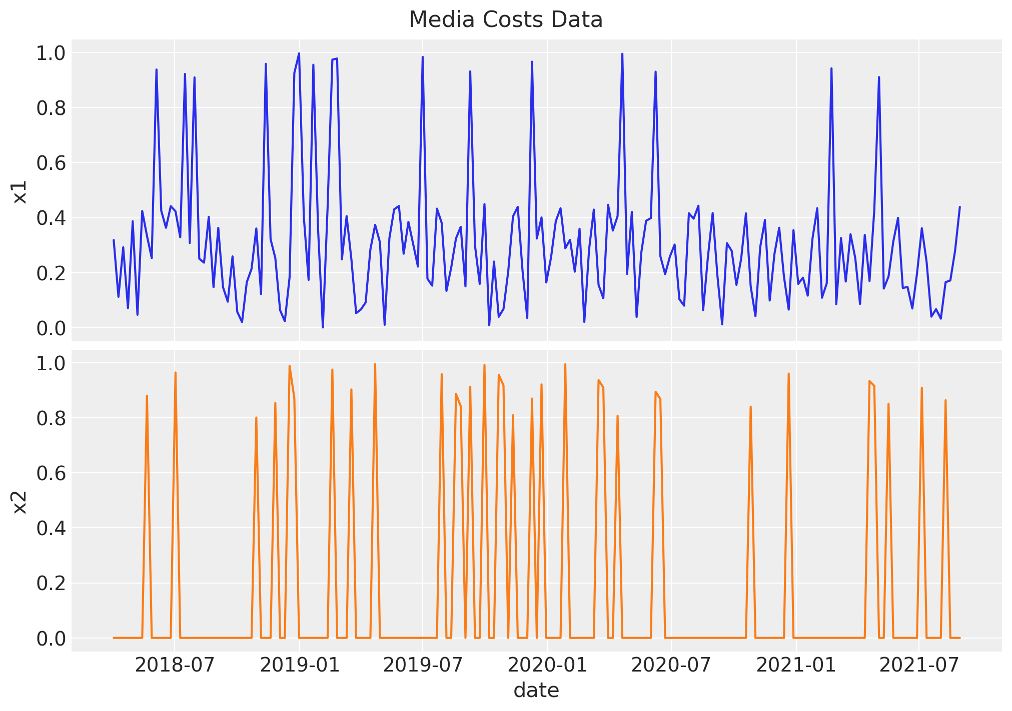
Now we generate synthetic data from two channels \(x_1\) and \(x_2\). We refer to it as the raw signal as it is going to be the input at the modeling phase. We expect the contribution of each channel to be different, based on the carryover and saturation parameters.

Raw Signal

# media data
x1 = rng.uniform(low=0.0, high=1.0, size=n)
df["x1"] = np.where(x1 > 0.9, x1, x1 / 2)

x2 = rng.uniform(low=0.0, high=1.0, size=n)
df["x2"] = np.where(x2 > 0.8, x2, 0)


fig, ax = plt.subplots(
    nrows=2, ncols=1, figsize=(10, 7), sharex=True, sharey=True, layout="constrained"
)
sns.lineplot(x="date_week", y="x1", data=df, color="C0", ax=ax[0])
sns.lineplot(x="date_week", y="x2", data=df, color="C1", ax=ax[1])
ax[1].set(xlabel="date")
fig.suptitle("Media Costs Data", fontsize=16);

../../_images/b3593754ed6cb5fc4771944964c9c024ea2b9057373f846634031bf8a311259b.png

Remark: By design, \(x_{1}\) should resemble a typical paid social channel and \(x_{2}\) a offline (e.g. TV) spend time series.

Effect Signal

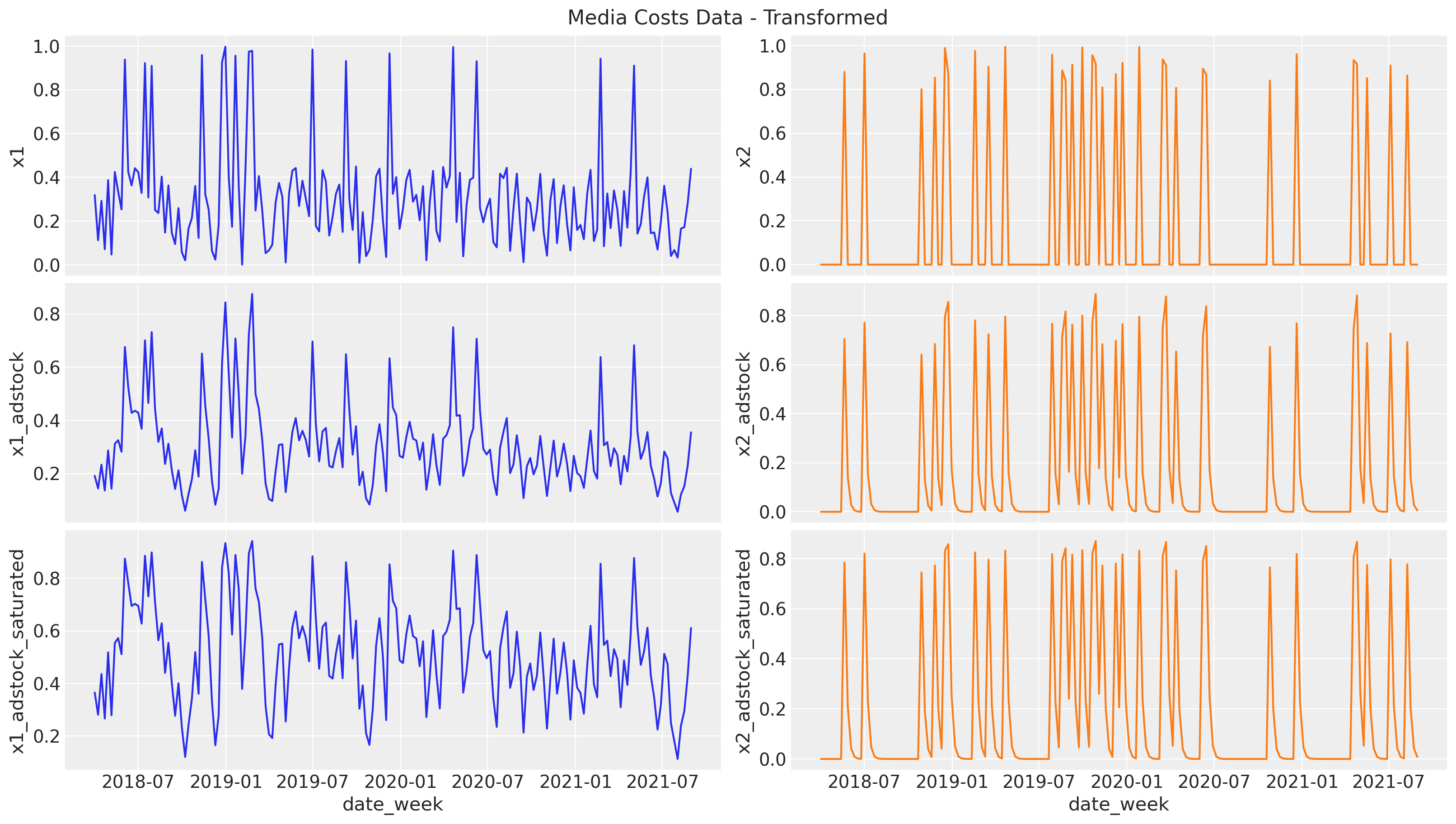
Next, we pass the raw signal through the two transformations: first the geometric adstock (carryover effect) and then the logistic saturation. Note that we set the parameters ourselves, but we will recover them back from the model.

Let’s start with the adstock transformation. We set the adstock parameter \(0 < \alpha < 1\) to be \(0.4\) and \(0.2\) for \(x_1\) and \(x_2\) respectively. We set a maximum lag effect of \(8\) weeks.

# apply geometric adstock transformation
alpha1: float = 0.4
alpha2: float = 0.2

df["x1_adstock"] = (
    geometric_adstock(x=df["x1"].to_numpy(), alpha=alpha1, l_max=8, normalize=True)
    .eval()
    .flatten()
)

df["x2_adstock"] = (
    geometric_adstock(x=df["x2"].to_numpy(), alpha=alpha2, l_max=8, normalize=True)
    .eval()
    .flatten()
)

Next, we compose the resulting adstock signals with the logistic saturation function. We set the parameter \(\lambda > 0\) to be \(4\) and \(3\) for \(z_1\) and \(z_2\) respectively.

# apply saturation transformation
lam1: float = 4.0
lam2: float = 3.0

df["x1_adstock_saturated"] = logistic_saturation(
    x=df["x1_adstock"].to_numpy(), lam=lam1
).eval()

df["x2_adstock_saturated"] = logistic_saturation(
    x=df["x2_adstock"].to_numpy(), lam=lam2
).eval()

We can now visualize the effect signal for each channel after each transformation:

fig, ax = plt.subplots(
    nrows=3, ncols=2, figsize=(16, 9), sharex=True, sharey=False, layout="constrained"
)
sns.lineplot(x="date_week", y="x1", data=df, color="C0", ax=ax[0, 0])
sns.lineplot(x="date_week", y="x2", data=df, color="C1", ax=ax[0, 1])
sns.lineplot(x="date_week", y="x1_adstock", data=df, color="C0", ax=ax[1, 0])
sns.lineplot(x="date_week", y="x2_adstock", data=df, color="C1", ax=ax[1, 1])
sns.lineplot(x="date_week", y="x1_adstock_saturated", data=df, color="C0", ax=ax[2, 0])
sns.lineplot(x="date_week", y="x2_adstock_saturated", data=df, color="C1", ax=ax[2, 1])
fig.suptitle("Media Costs Data - Transformed", fontsize=16);

../../_images/12d44196dd2036a04e39724f7b540dfbde550811696b91a0ac1780d4a13bbc7a.png

3. Trend & Seasonal Components#

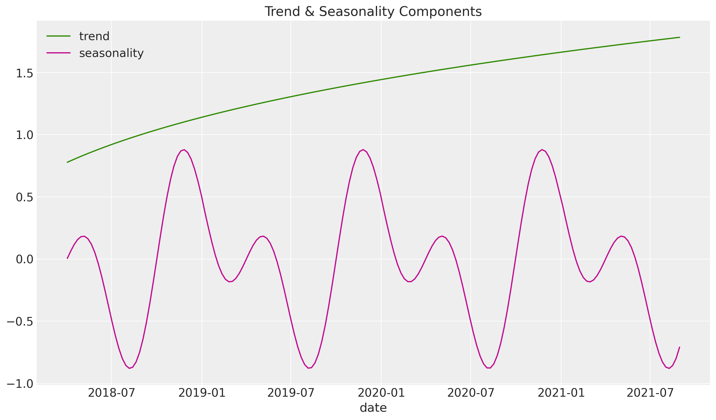
Now we add synthetic trend and seasonal components to the effect signal.

df["trend"] = (np.linspace(start=0.0, stop=50, num=n) + 10) ** (1 / 4) - 1

df["cs"] = -np.sin(2 * 2 * np.pi * df["dayofyear"] / 365.5)
df["cc"] = np.cos(1 * 2 * np.pi * df["dayofyear"] / 365.5)
df["seasonality"] = 0.5 * (df["cs"] + df["cc"])

fig, ax = plt.subplots()
sns.lineplot(x="date_week", y="trend", color="C2", label="trend", data=df, ax=ax)
sns.lineplot(
    x="date_week", y="seasonality", color="C3", label="seasonality", data=df, ax=ax
)
ax.legend(loc="upper left")
ax.set(title="Trend & Seasonality Components", xlabel="date", ylabel=None);

../../_images/ff8ca1e7b7f94715b73137dc458a29b343b458a4a8f76ce5e8977338a6145d4a.png

4. Control Variables#

We add two events where there was a remarkable peak in our target variable. We assume they are independent an not seasonal (e.g. launch of a particular product).

df["event_1"] = (df["date_week"] == "2019-05-13").astype(float)
df["event_2"] = (df["date_week"] == "2020-09-14").astype(float)

5. Target Variable#

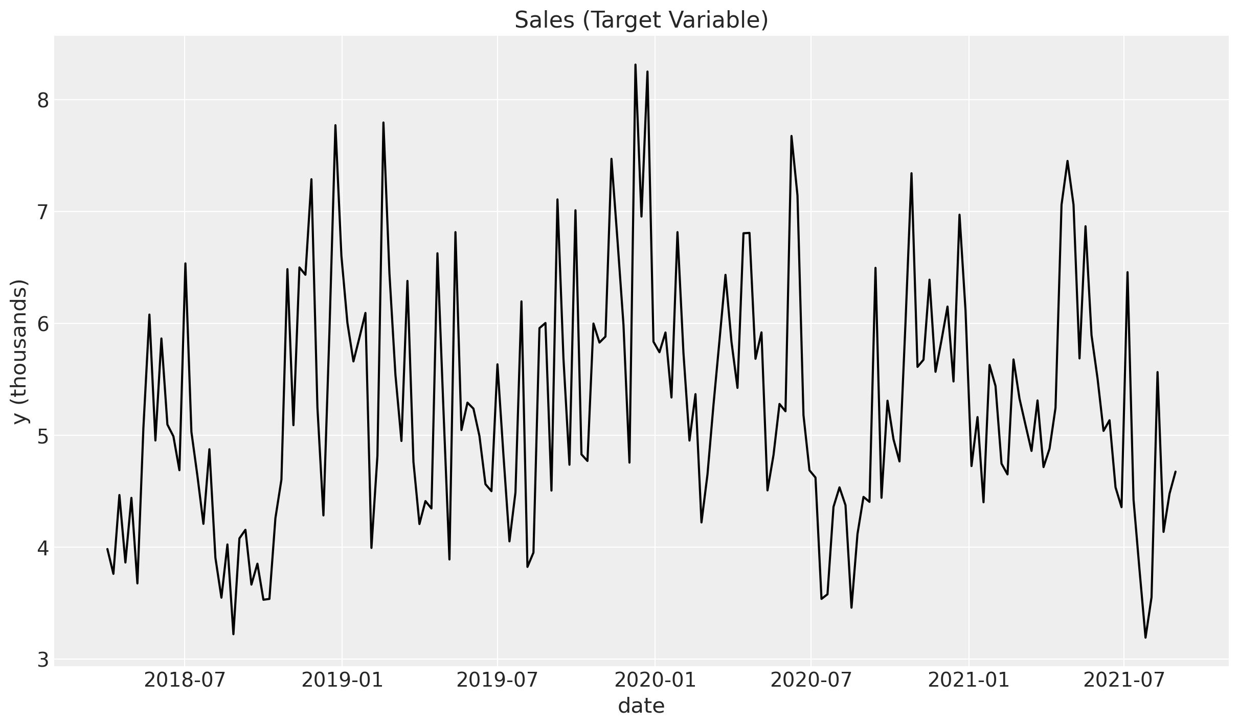
Finally, we define the target variable (sales) \(y\). We assume it is a linear combination of the effect signal, the trend and the seasonal components, plus the two events and an intercept. We also add some Gaussian noise.

df["intercept"] = 2.0
df["epsilon"] = rng.normal(loc=0.0, scale=0.25, size=n)

amplitude = 1
beta_1 = 3.0
beta_2 = 2.0
betas = [beta_1, beta_2]


df["y"] = amplitude * (
    df["intercept"]
    + df["trend"]
    + df["seasonality"]
    + 1.5 * df["event_1"]
    + 2.5 * df["event_2"]
    + beta_1 * df["x1_adstock_saturated"]
    + beta_2 * df["x2_adstock_saturated"]
    + df["epsilon"]
)

fig, ax = plt.subplots()
sns.lineplot(x="date_week", y="y", color="black", data=df, ax=ax)
ax.set(title="Sales (Target Variable)", xlabel="date", ylabel="y (thousands)");

../../_images/6caf59a4cecc648d8918b80b7cf125d2f111d2dd246405f05c877b95df3af7e7.png

6. Media Contribution Interpretation#

From the data generating process we can compute the relative contribution of each channel to the target variable. We will recover these values back from the model.

contribution_share_x1: float = (beta_1 * df["x1_adstock_saturated"]).sum() / (
    beta_1 * df["x1_adstock_saturated"] + beta_2 * df["x2_adstock_saturated"]
).sum()

contribution_share_x2: float = (beta_2 * df["x2_adstock_saturated"]).sum() / (
    beta_1 * df["x1_adstock_saturated"] + beta_2 * df["x2_adstock_saturated"]
).sum()

print(f"Contribution Share of x1: {contribution_share_x1:.2f}")
print(f"Contribution Share of x2: {contribution_share_x2:.2f}")

Contribution Share of x1: 0.81
Contribution Share of x2: 0.19

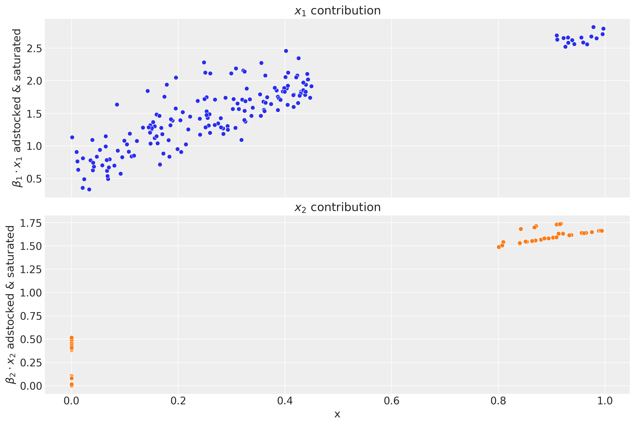
We can obtain the contribution plots for each channel where we clearly see the effect of the adstock and saturation transformations.

fig, ax = plt.subplots(
    nrows=2, ncols=1, figsize=(12, 8), sharex=True, sharey=False, layout="constrained"
)

for i, x in enumerate(["x1", "x2"]):
    sns.scatterplot(
        x=df[x],
        y=amplitude * betas[i] * df[f"{x}_adstock_saturated"],
        color=f"C{i}",
        ax=ax[i],
    )
    ax[i].set(
        title=f"$x_{i + 1}$ contribution",
        ylabel=f"$\\beta_{i + 1} \\cdot x_{i + 1}$ adstocked & saturated",
        xlabel="x",
    )

../../_images/e2f8505482cf148e2d644dc995849ff0a0a25056ae59b51b3d3de0e2b1061dca.png

This plot shows some interesting aspects of the media contribution:

The adstock effect is reflected in the non-zero contribution of the channel even when the spend is zero.
One clearly see the saturation effect as the contribution growth (slope) decreases as the spend increases.

As we will see in Part II of this notebook, we will recover these plots from the model!

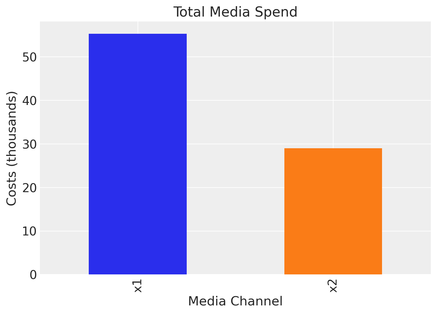
We see that channel \(x_{1}\) has a higher contribution than \(x_{2}\). This could be explained by the fact that there was more spend in channel \(x_{1}\) than in channel \(x_{2}\):

fig, ax = plt.subplots(figsize=(7, 5))
df[["x1", "x2"]].sum().plot(kind="bar", color=["C0", "C1"], ax=ax)
ax.set(title="Total Media Spend", xlabel="Media Channel", ylabel="Costs (thousands)");

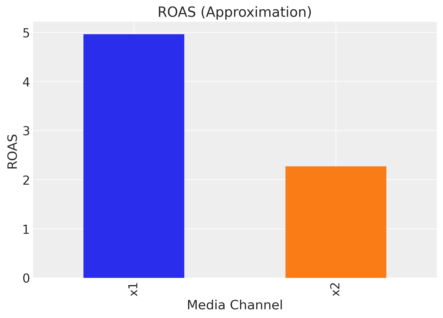
../../_images/018380c4ecc6b9509df19c71c4b3356b4b0694ea2b0c63f7812fc30f1402624a.png

However, one usually is not only interested in the contribution itself but rather the Return on Ad Spend (ROAS). That is, the contribution divided by the cost. We can compute the ROAS for each channel as follows:

roas_1 = (amplitude * beta_1 * df["x1_adstock_saturated"]).sum() / df["x1"].sum()
roas_2 = (amplitude * beta_2 * df["x2_adstock_saturated"]).sum() / df["x2"].sum()

fig, ax = plt.subplots(figsize=(7, 5))
(
    pd.Series(data=[roas_1, roas_2], index=["x1", "x2"]).plot(
        kind="bar", color=["C0", "C1"]
    )
)

ax.set(title="ROAS (Approximation)", xlabel="Media Channel", ylabel="ROAS");

../../_images/90b308d83d7dc4b63bbe77ad9f562473ee3df0f011cc72f9194c6cc500518769.png

That is, channel \(x_{1}\) seems to be more efficient than channel \(x_{2}\).

Remark: We recommended reading Section 4.1 in Jin, Yuxue, et al. “Bayesian methods for media mix modeling with carryover and shape effects.” (2017) for a detailed explanation of the ROAS (and mROAS). In particular:

If we transform our target variable \(y\) (e.g. with a log transformation), one needs to be careful with the ROAS computation as setting the spend to zero does not commute with the transformation.
One has to be careful with the adstock effect so that we include a carryover period to fully account for the effect of the spend. The ROAS estimation above is an approximation.

7. Data Output#

We of course will not have all of these features in our real data. Let’s filter out the features we will use for modeling:

columns_to_keep = [
    "date_week",
    "y",
    "x1",
    "x2",
    "event_1",
    "event_2",
    "dayofyear",
]

data = df[columns_to_keep].copy()

data.head()

	date_week	y	x1	dayofyear
0	2018-04-02	3.984662	0.318580	92
1	2018-04-09	3.762872	0.112388	99
2	2018-04-16	4.466967	0.292400	106
3	2018-04-23	3.864219	0.071399	113
4	2018-04-30	4.441625	0.386745	120

Part II: Modeling#

On this second part, we focus on the modeling process. We will use the data generated in Part I.

1. Feature Engineering#

Assuming we did an EDA and we have a good understanding of the data (we did not do it here as we generated the data ourselves, but please never skip the EDA!), we can start building our model. One thing we immediately see is the seasonality and the trend component. We can generate features ourselves as control variables, for example using a uniformly increasing straight line to model the trend component. In addition, we include dummy variables to encode the event_1 and event_2 contributions.

For the seasonality component we use Fourier modes (similar as in Prophet). We do not need to add the Fourier modes by hand as they are handled by the model API through the yearly_seasonality argument (see below). We use 4 modes for the seasonality component.

# trend feature
data["t"] = range(n)

data.head()

	date_week	y	x1	dayofyear	t
0	2018-04-02	3.984662	0.318580	92	0
1	2018-04-09	3.762872	0.112388	99	1
2	2018-04-16	4.466967	0.292400	106	2
3	2018-04-23	3.864219	0.071399	113	3
4	2018-04-30	4.441625	0.386745	120	4

2. Model Specification#

We can specify the model structure using the DelayedSaturatedMMM class. This class, handles a lot of internal boilerplate code for us such us scaling the data (see details below) and handy diagnostics and reporting plots. One great feature is that we can specify the channel priors distributions ourselves, which fundamental component of the bayesian workflow as we can incorporate our prior knowledge into the model. This is one of the most important advantages of using a bayesian approach. Let’s see how we can do it.

As we do not know much more about the channels, we start with a simple heuristic:

The channel contributions should be positive, so we can for example use a HalfNormal distribution as prior. We need to set the sigma parameter per channel. The higher the sigma, the more “freedom” it has to fit the data. To specify sigma we can use the following point.
We expect channels where we spend the most to have more attributed sales , before seeing the data. This is a very reasonable assumption (note that we are not imposing anything at the level of efficiency!).

How to incorporate this heuristic into the model? To begin with, it is important to note that the DelayedSaturatedMMM class scales the target and input variables through an MaxAbsScaler transformer from scikit-learn, its important to specify the priors in the scaled space (i.e. between 0 and 1). One way to do it is to use the spend share as the sigma parameter for the HalfNormal distribution. We can actually add a scaling factor to take into account the support of the distribution.

First, let’s compute the share of spend per channel:

total_spend_per_channel = data[["x1", "x2"]].sum(axis=0)

spend_share = total_spend_per_channel / total_spend_per_channel.sum()

spend_share

x1    0.65632
x2    0.34368
dtype: float64

Next, we specify the sigma parameter per channel:

# The scale necessary to make a HalfNormal distribution have unit variance
HALFNORMAL_SCALE = 1 / np.sqrt(1 - 2 / np.pi)

n_channels = 2

prior_sigma = HALFNORMAL_SCALE * n_channels * spend_share.to_numpy()

prior_sigma.tolist()

[2.1775326025486734, 1.1402608773919387]

Delayed Saturated MMM follows sklearn convention, so we need to split our data into X (predictors) and y(target value)

X = data.drop("y", axis=1)
y = data["y"]

You can use the optional parameter ‘model_config’ to apply your own priors to the model. Each entry in the ‘model_config’ contains a key that corresponds to a registered distribution name in our model. The value of the key is a dictionary that describes the input parameters of that specific distribution.

If you’re unsure how to define your own priors, you can use the ‘default_model_config’ property of DelayedSaturatedMMM to see the required structure.

dummy_model = DelayedSaturatedMMM(date_column="", channel_columns="", adstock_max_lag=4)
dummy_model.default_model_config

{'intercept': {'dist': 'Normal', 'kwargs': {'mu': 0, 'sigma': 2}},
 'beta_channel': {'dist': 'HalfNormal', 'kwargs': {'sigma': 2}},
 'alpha': {'dist': 'Beta', 'kwargs': {'alpha': 1, 'beta': 3}},
 'lam': {'dist': 'Gamma', 'kwargs': {'alpha': 3, 'beta': 1}},
 'likelihood': {'dist': 'Normal',
  'kwargs': {'sigma': {'dist': 'HalfNormal', 'kwargs': {'sigma': 2}}}},
 'gamma_control': {'dist': 'Normal', 'kwargs': {'mu': 0, 'sigma': 2}},
 'gamma_fourier': {'dist': 'Laplace', 'kwargs': {'mu': 0, 'b': 1}}}

You can change only the prior parameters that you wish, no need to alter all of them, unless you’d like to!

my_model_config = {
    "beta_channel": {
        "dist": "LogNormal",
        "kwargs": {"mu": np.array([2, 1]), "sigma": prior_sigma},
    },
    "likelihood": {
        "dist": "Normal",
        "kwargs": {
            "sigma": {"dist": "HalfNormal", "kwargs": {"sigma": 2}}
            # Also possible define sigma as:
            # {'sigma': 5}
        },
    },
}

Remark: For the prior specification there is no right or wrong answer. It all depends on the data, the context and the assumptions you are willing to make. It is always recommended to do some prior predictive sampling and sensitivity analysis to check the impact of the priors on the posterior. We skip this here for the sake of simplicity. If you are not sure about specific priors, the DelayedSaturatedMMM class has some default priors that you can use as a starting point.

Model sampler allows specifying set of parameters that will be passed to fit the same way as the kwargs are getting passed so far. It doesn’t disable the fit kwargs, but rather extend them, to enable customizable and preservable configuration. By default the sampler_config for DelayedSaturatedMMM is empty. But if you’d like to use it, you can define it like showed below:

my_sampler_config = {"progressbar": True}

Now we are ready to use the DelayedSaturatedMMM class to define the model.

mmm = DelayedSaturatedMMM(
    model_config=my_model_config,
    sampler_config=my_sampler_config,
    date_column="date_week",
    channel_columns=["x1", "x2"],
    control_columns=[
        "event_1",
        "event_2",
        "t",
    ],
    adstock_max_lag=8,
    yearly_seasonality=2,
)

Observe how the media transformations were handled by the class DelayedSaturatedMMM.

4. Model Diagnostics#

The fit_result attribute contains the pymc trace object.

We can therefore use all the pymc machinery to run model diagnostics. First, let’s see the summary of the trace:

az.summary(
    data=mmm.fit_result,
    var_names=[
        "intercept",
        "likelihood_sigma",
        "beta_channel",
        "alpha",
        "lam",
        "gamma_control",
        "gamma_fourier",
    ],
)

	mean	sd	hdi_3%	hdi_97%	mcse_mean	mcse_sd	ess_bulk	ess_tail	r_hat
intercept	0.350	0.013	0.324	0.374	0.000	0.000	2563.0	2628.0	1.0
likelihood_sigma	0.030	0.002	0.027	0.033	0.000	0.000	4380.0	2885.0	1.0
beta_channel[x1]	0.361	0.019	0.328	0.399	0.000	0.000	2101.0	2424.0	1.0
beta_channel[x2]	0.288	0.148	0.193	0.426	0.006	0.004	1134.0	816.0	1.0
alpha[x1]	0.396	0.031	0.333	0.448	0.001	0.000	2595.0	2826.0	1.0
alpha[x2]	0.197	0.040	0.120	0.269	0.001	0.001	2041.0	1885.0	1.0
lam[x1]	4.076	0.371	3.370	4.760	0.007	0.005	3214.0	2466.0	1.0
lam[x2]	3.023	1.199	0.796	5.188	0.033	0.023	1162.0	829.0	1.0
gamma_control[event_1]	0.246	0.031	0.187	0.306	0.000	0.000	5741.0	2721.0	1.0
gamma_control[event_2]	0.328	0.032	0.268	0.387	0.000	0.000	5151.0	2832.0	1.0
gamma_control[t]	0.001	0.000	0.001	0.001	0.000	0.000	3311.0	3027.0	1.0
gamma_fourier[sin_order_1]	0.003	0.003	-0.003	0.010	0.000	0.000	4547.0	2957.0	1.0
gamma_fourier[cos_order_1]	0.063	0.003	0.057	0.069	0.000	0.000	5607.0	2819.0	1.0
gamma_fourier[sin_order_2]	-0.057	0.003	-0.064	-0.051	0.000	0.000	4015.0	2826.0	1.0
gamma_fourier[cos_order_2]	0.002	0.003	-0.005	0.008	0.000	0.000	3997.0	2839.0	1.0

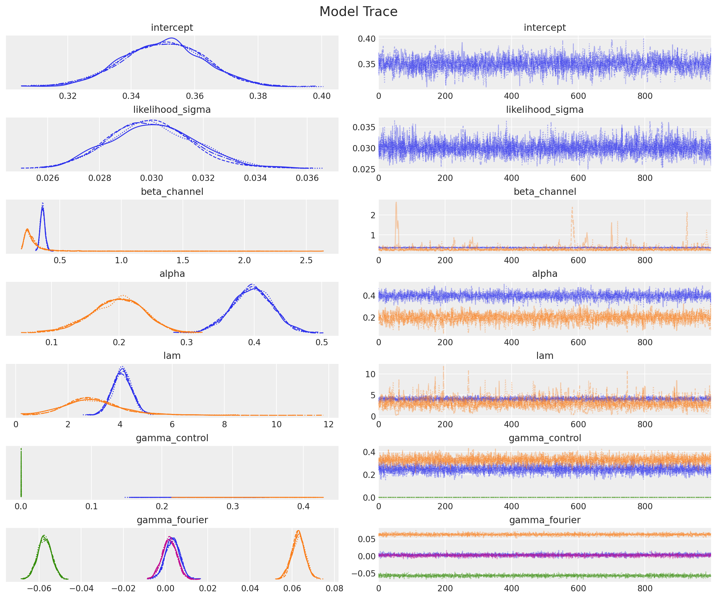
Observe that the estimated parameters for \(\alpha\) and \(\lambda\) are very close to the ones we set in the data generation process! Let’s plot the trace for the parameters:

_ = az.plot_trace(
    data=mmm.fit_result,
    var_names=[
        "intercept",
        "likelihood_sigma",
        "beta_channel",
        "alpha",
        "lam",
        "gamma_control",
        "gamma_fourier",
    ],
    compact=True,
    backend_kwargs={"figsize": (12, 10), "layout": "constrained"},
)
plt.gcf().suptitle("Model Trace", fontsize=16);

../../_images/82d5bed070d0d1e99122ae482440ba2c5b1fcc8a68eaf7bf763b2cb408cd15c3.png

Now we sample from the posterior predictive distribution:

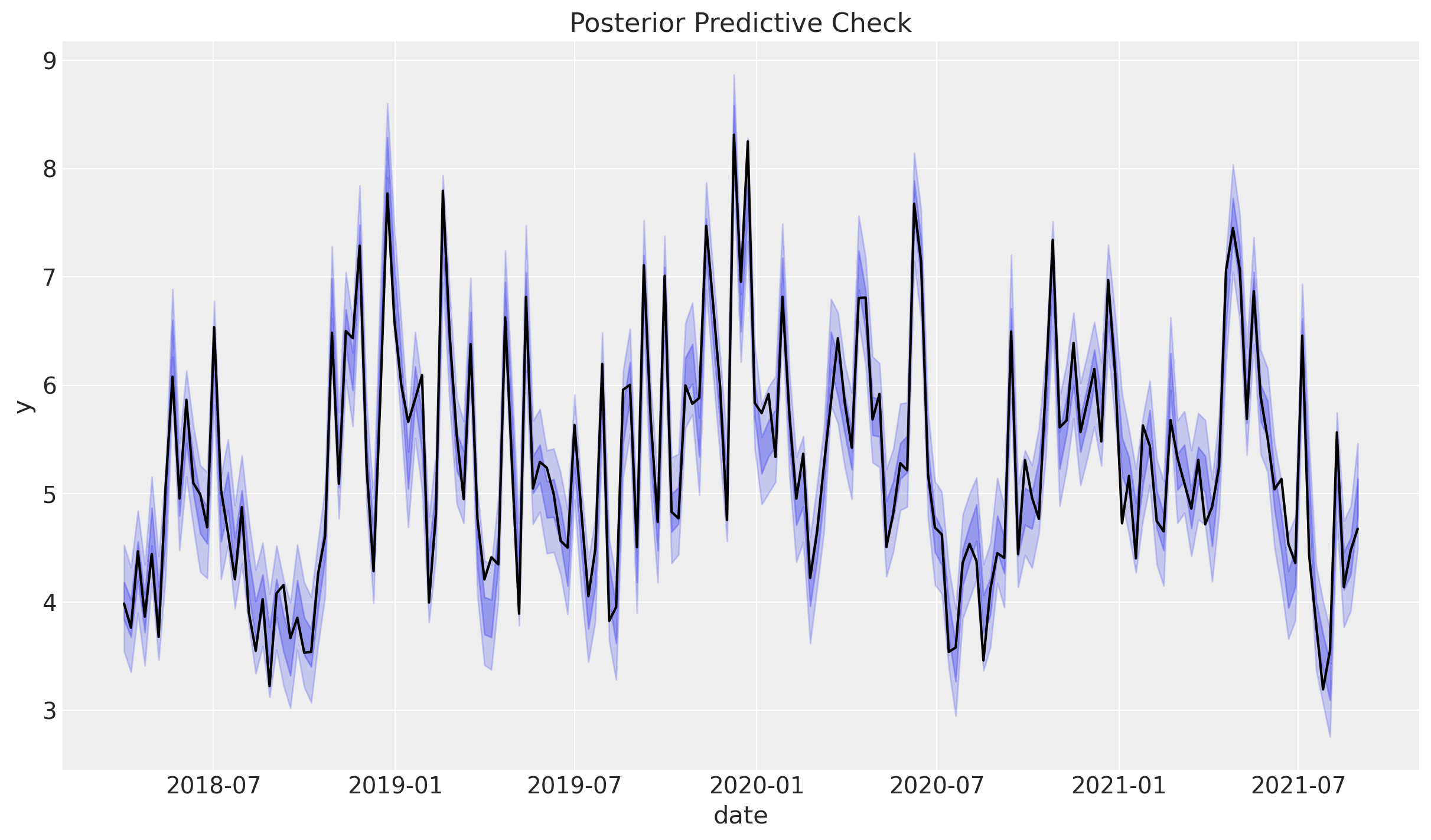
We can now plot the posterior predictive distribution for the target variable:

mmm.plot_posterior_predictive(original_scale=True);

../../_images/314ef7999df18b144a44aabe2945c66d204a43cd4f6843a495e9364e628ebe96.png

The fit looks very good (as expected)!

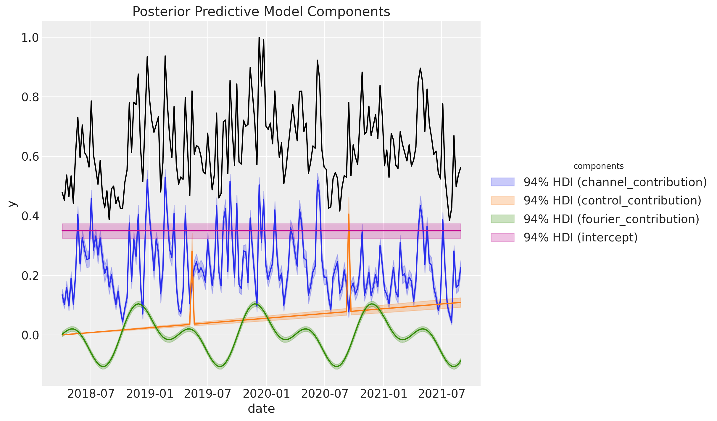
We can decompose the posterior predictive distribution into the different components:

mmm.plot_components_contributions();

../../_images/1d685005927e3f0fc34557fe730fa87becf7690ae6fc8db00c058fbc276e2035.png

Remark: This plot shows the decomposition of the normalized target variable when by dividing by its maximum value. Do not forget that internally we are scaling the variables to make the model sample more efficiently. You can recover the transformations from the API methods, e.g.

mmm.get_target_transformer()

Pipeline(steps=[('scaler', MaxAbsScaler())])

In a Jupyter environment, please rerun this cell to show the HTML representation or trust the notebook.
On GitHub, the HTML representation is unable to render, please try loading this page with nbviewer.org.

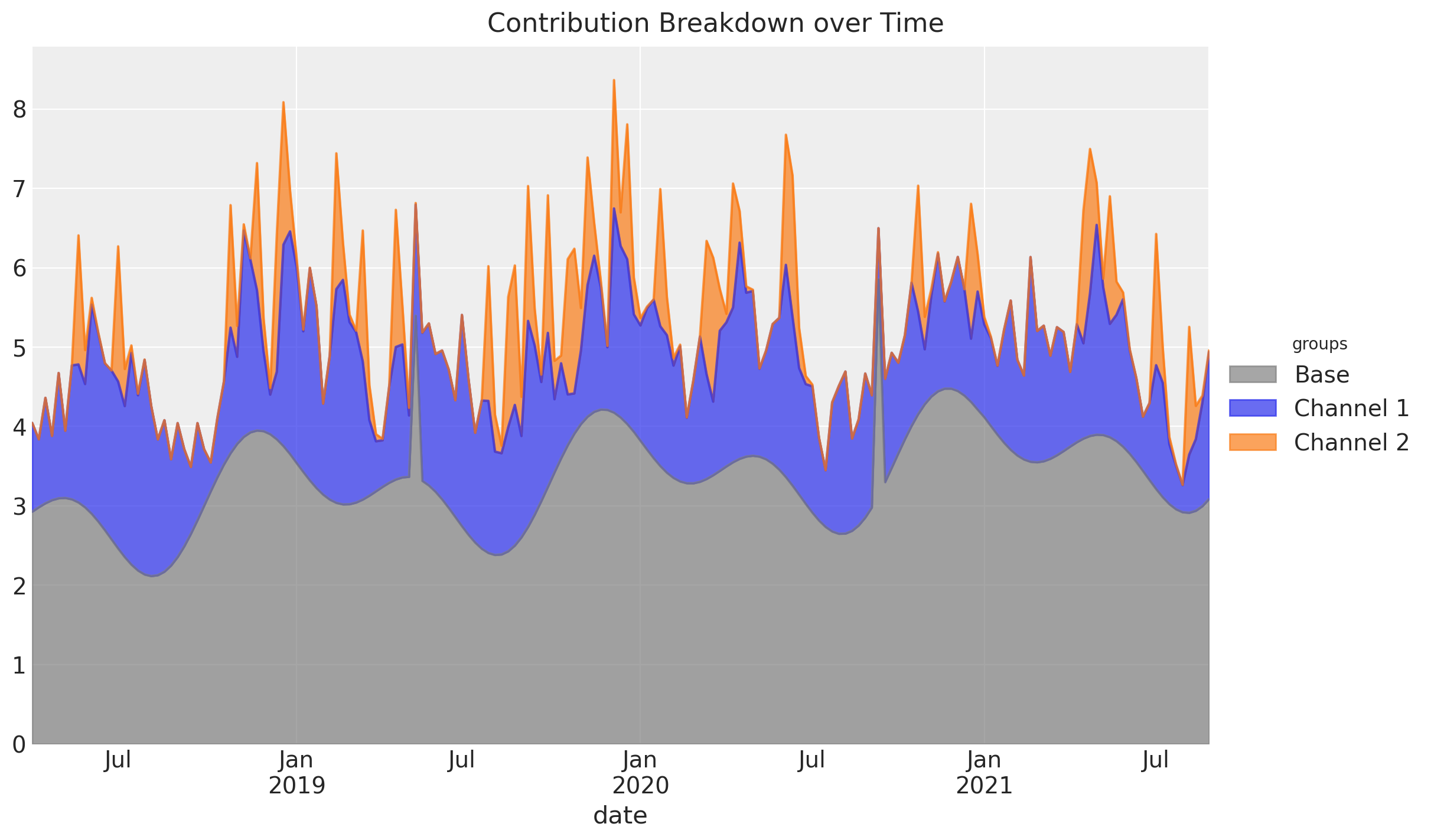
A similar decomposition can be achieved using an area plot:

groups = {
    "Base": [
        "intercept",
        "event_1",
        "event_2",
        "t",
        "sin_order_1",
        "sin_order_2",
        "cos_order_1",
        "cos_order_2",
    ],
    "Channel 1": ["x1"],
    "Channel 2": ["x2"],
}

fig = mmm.plot_grouped_contribution_breakdown_over_time(
    stack_groups=groups,
    original_scale=True,
    area_kwargs={
        "color": {
            "Channel 1": "C0",
            "Channel 2": "C1",
            "Base": "gray",
            "Seasonality": "black",
        },
        "alpha": 0.7,
    },
)

fig.suptitle("Contribution Breakdown over Time", fontsize=16);

../../_images/fcb5e641e022a3e82cafacc70fd3142ea13baf55bb396ff17c8e21bc67234d1e.png

Note that this only works if the contributions of the channel or control variable are strictly positive.

We can extract the all the input variables contributions over time, i.e. the regression coefficients times the feature values, as follows:

get_mean_contributions_over_time_df = mmm.compute_mean_contributions_over_time(
    original_scale=True
)

get_mean_contributions_over_time_df.head()

	x1	x2	event_1	event_2	t	sin_order_1	cos_order_1	sin_order_2	cos_order_2	intercept
date
2018-04-02	1.118764	0.0	0.0	0.0	0.000000	0.027485	-0.006193	0.011271	-0.015895	2.909302
2018-04-09	0.855933	0.0	0.0	0.0	0.005089	0.027247	-0.069047	0.124574	-0.015346	2.909302
2018-04-16	1.328675	0.0	0.0	0.0	0.010178	0.026614	-0.130901	0.230687	-0.013912	2.909302
2018-04-23	0.809616	0.0	0.0	0.0	0.015267	0.025596	-0.190859	0.323484	-0.011675	2.909302
2018-04-30	1.578756	0.0	0.0	0.0	0.020356	0.024207	-0.248053	0.397610	-0.008764	2.909302

5. Media Parameters#

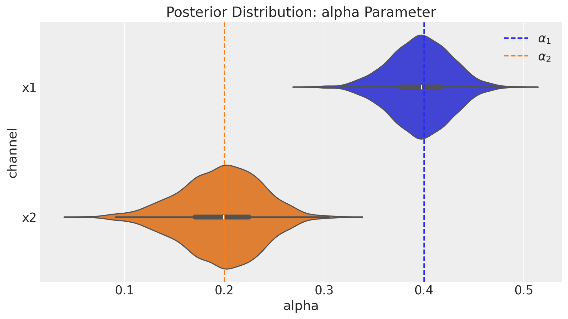
We can deep-dive into the media transformation parameters. We want to compare the posterior distributions against the true values.

fig = mmm.plot_channel_parameter(param_name="alpha", figsize=(9, 5))
ax = fig.axes[0]
ax.axvline(x=alpha1, color="C0", linestyle="--", label=r"$\alpha_1$")
ax.axvline(x=alpha2, color="C1", linestyle="--", label=r"$\alpha_2$")
ax.legend(loc="upper right");

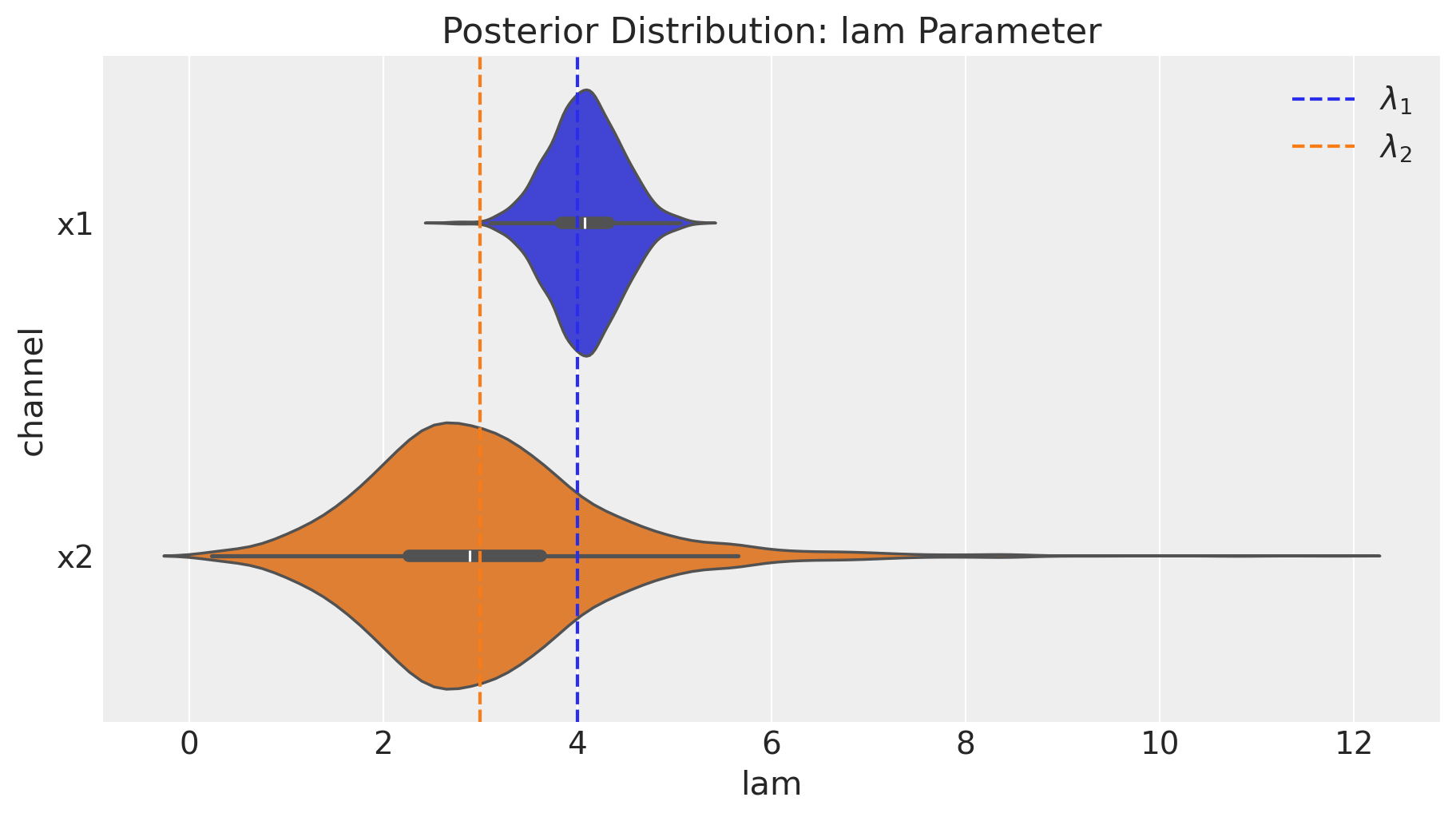
../../_images/72d5b64ec35efac6ab9972f09f0a3a15eeb2f71b3aebc328393e3e0dacfce3b9.png

fig = mmm.plot_channel_parameter(param_name="lam", figsize=(9, 5))
ax = fig.axes[0]
ax.axvline(x=lam1, color="C0", linestyle="--", label=r"$\lambda_1$")
ax.axvline(x=lam2, color="C1", linestyle="--", label=r"$\lambda_2$")
ax.legend(loc="upper right");

../../_images/d7a66cc67253a56c4f548a25a0ccd2f0b28ea9b242e77697c742a454b17c3133.png

We indeed see that our media parameter were successfully recovered!

6. Media Deep-Dive#

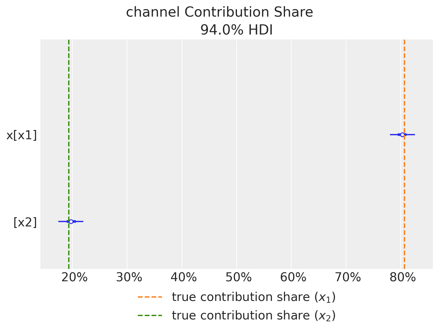
First we can compute the relative contribution of each channel to the target variable. Note that we recover the true values!

fig = mmm.plot_channel_contribution_share_hdi(figsize=(7, 5))
ax = fig.axes[0]
ax.axvline(
    x=contribution_share_x1,
    color="C1",
    linestyle="--",
    label="true contribution share ($x_1$)",
)
ax.axvline(
    x=contribution_share_x2,
    color="C2",
    linestyle="--",
    label="true contribution share ($x_2$)",
)
ax.legend(loc="upper center", bbox_to_anchor=(0.5, -0.05), ncol=1);

../../_images/d8406f9c7d1a437bd7ed88615e05dcbd5d73a2769f76671c9907a3acdf7df22d.png

Next, we can plot the relative contribution of each channel to the target variable.

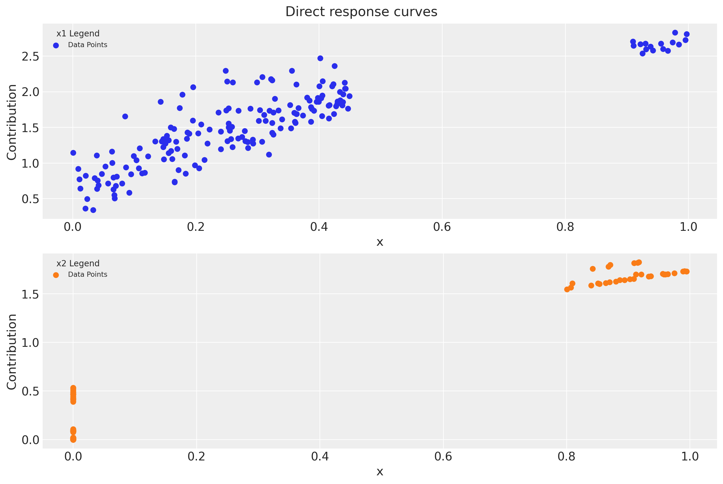
First we plot the direct contribution per channel. Again, we get very close values as the ones obtained in Part I.

fig = mmm.plot_direct_contribution_curves()
[ax.set(xlabel="x") for ax in fig.axes];

../../_images/e34f0ddbb8d87510c8dc3552cb165ba547cbca0c6c2d4db861bfe5b98581b58f.png

Note that trying to get the delayed cumulative contribution is not that easy as contributions from the past leak into the future. Specifically, note that we apply the saturation function to the aggregation. As the saturation function is non-linear. This is not the same as taking the sum of the saturation contributions Hence, is very hard to reverse engineer the contribution after carryover and saturation composition this way.

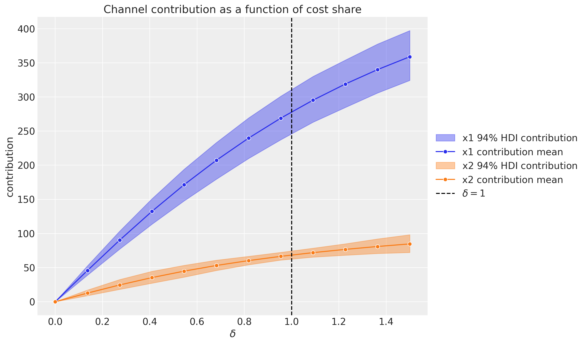
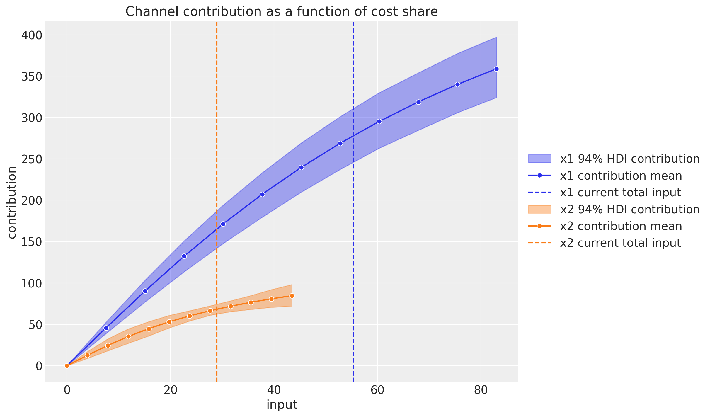
A more transparent alternative is to evaluate the channel contribution at different share spend levels for the complete training period. Concretely, if the denote by \(\delta\) the input channel data percentage level, so that for \(\delta = 1\) we have the model input spend data and for \(\delta = 1.5\) we have a \(50\%\) increase in the spend, then we can compute the channel contribution at a grid of \(\delta\)-values and plot the results:

mmm.plot_channel_contributions_grid(start=0, stop=1.5, num=12);

../../_images/873530cde8a7f45ce07dbd0410e1ebe5280cc67e2481066ed87523c6a4d2b02e.png

This plot does account for carryover (adstock) and saturation effects.
We see that when we have no spend, the contribution is zero (assuming there twas no spend in the past, otherwise the carryover effect would be non-zero).

Observe that these grid values serve as inputs for an optimization step.

We can also plot the same contribution using the x-axis as the total channel input (e.g. total spend in EUR).

mmm.plot_channel_contributions_grid(start=0, stop=1.5, num=12, absolute_xrange=True);

../../_images/472f299fa952ebb8fb609fe5803162c0c3235c19c35bbb6b1c3a69b3910ef1c1.png

7. Contribution Recovery#

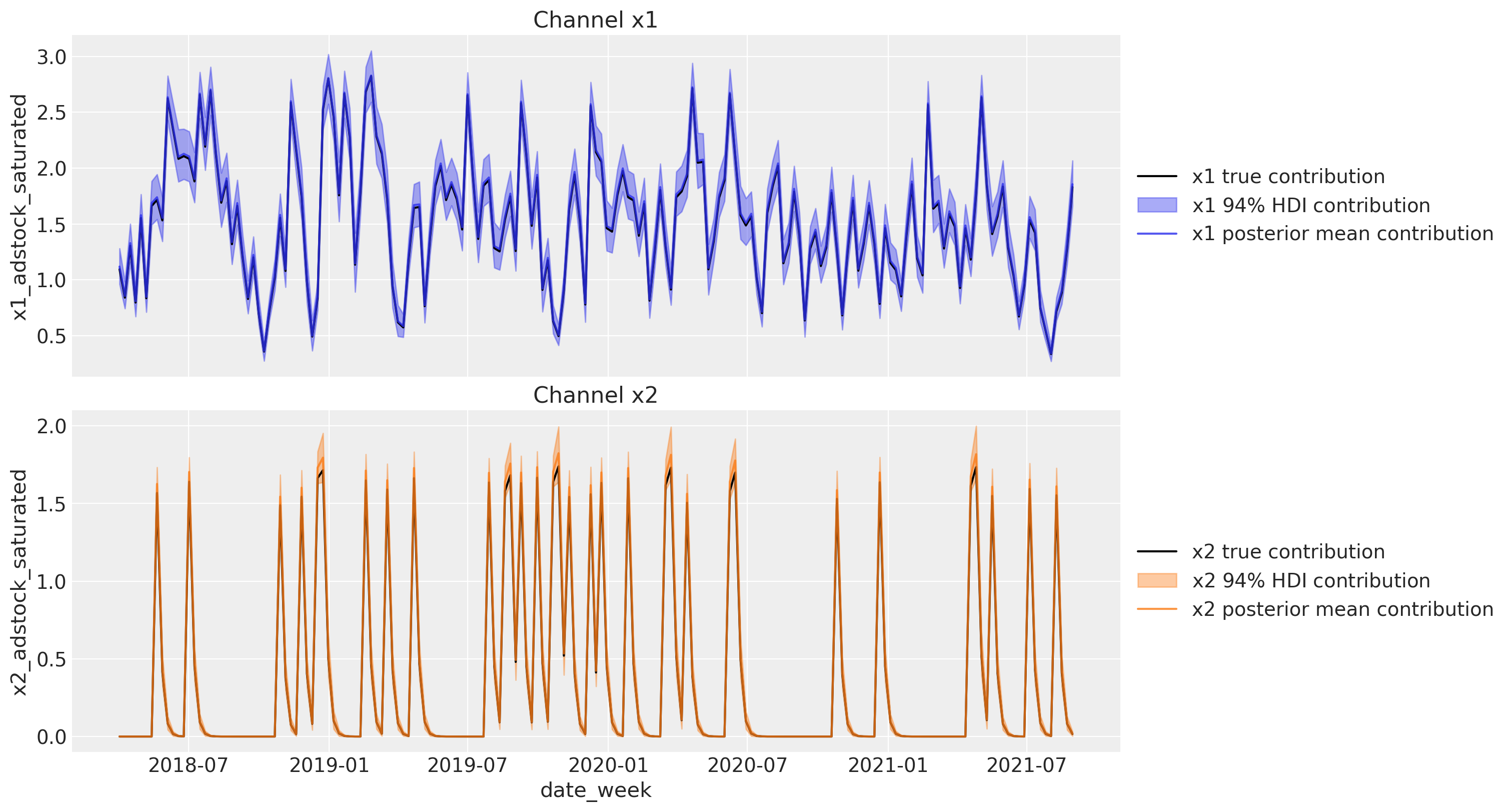
Next, we can plot the direct contribution of each channel to the target variable over time.

channels_contribution_original_scale = mmm.compute_channel_contribution_original_scale()
channels_contribution_original_scale_hdi = az.hdi(
    ary=channels_contribution_original_scale
)

fig, ax = plt.subplots(
    nrows=2, figsize=(15, 8), ncols=1, sharex=True, sharey=False, layout="constrained"
)

for i, x in enumerate(["x1", "x2"]):
    # Estimate true contribution in the original scale from the data generating process
    sns.lineplot(
        x=df["date_week"],
        y=amplitude * betas[i] * df[f"{x}_adstock_saturated"],
        color="black",
        label=f"{x} true contribution",
        ax=ax[i],
    )
    # HDI estimated contribution in the original scale
    ax[i].fill_between(
        x=df["date_week"],
        y1=channels_contribution_original_scale_hdi.sel(channel=x)["x"][:, 0],
        y2=channels_contribution_original_scale_hdi.sel(channel=x)["x"][:, 1],
        color=f"C{i}",
        label=rf"{x} $94\%$ HDI contribution",
        alpha=0.4,
    )
    # Mean estimated contribution in the original scale
    sns.lineplot(
        x=df["date_week"],
        y=get_mean_contributions_over_time_df[x].to_numpy(),
        color=f"C{i}",
        label=f"{x} posterior mean contribution",
        alpha=0.8,
        ax=ax[i],
    )
    ax[i].legend(loc="center left", bbox_to_anchor=(1, 0.5))
    ax[i].set(title=f"Channel {x}")

../../_images/09d967ba52fc3172f908334d8d6a9fbe0cd02d2c3f67f400015c07ae2fc8a9d7.png

The results look great! We therefore successfully recovered the true values from the data generation process. We have also seen how easy is to use the DelayedSaturatedMMM class to fit media mix models! It takes over the model specification and the media transformations, while having all the flexibility of pymc!

8. ROAS#

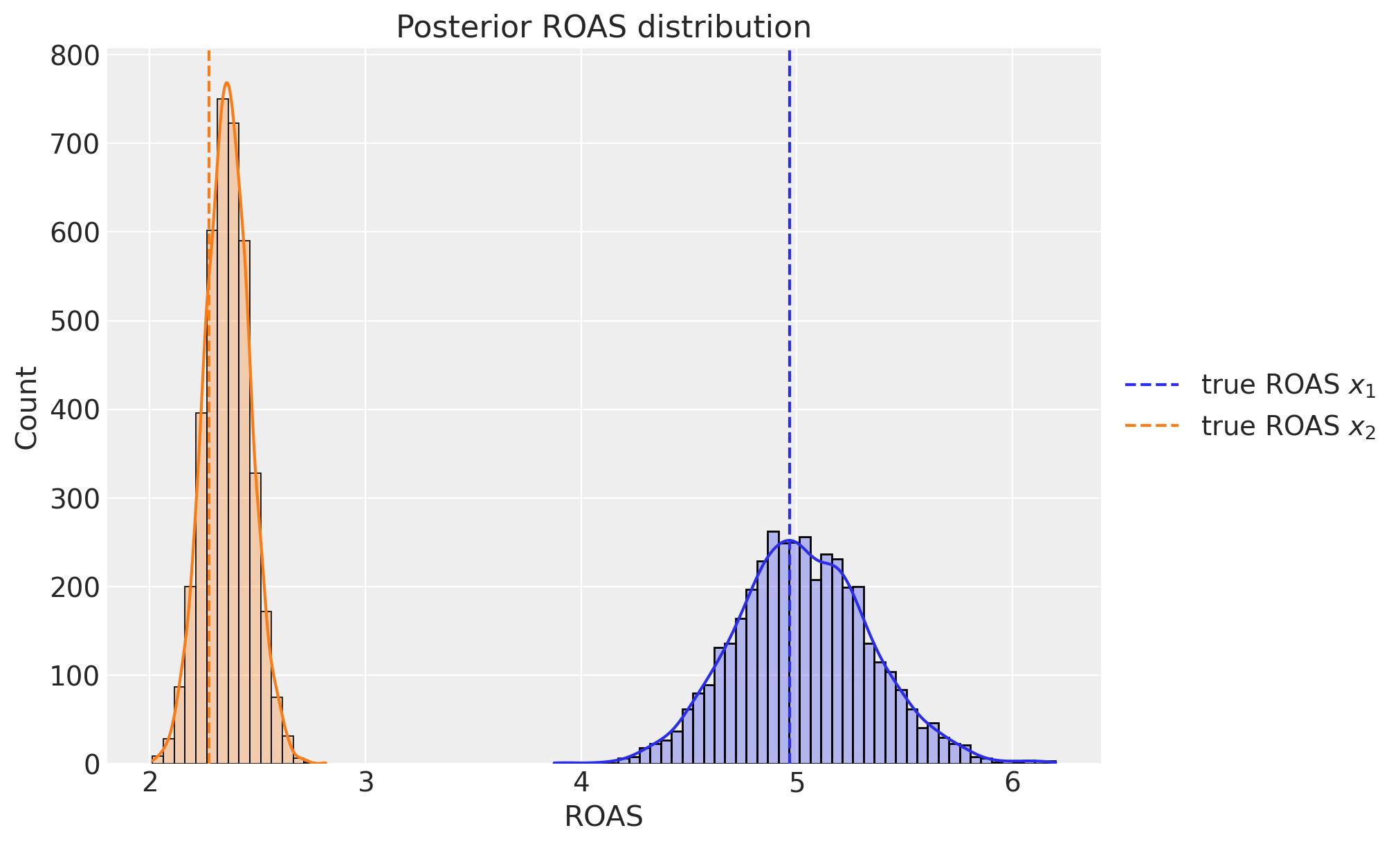
Finally, we can compute the (approximate) ROAS posterior distribution for each channel.

channel_contribution_original_scale = mmm.compute_channel_contribution_original_scale()

roas_samples = (
    channel_contribution_original_scale.stack(sample=("chain", "draw")).sum("date")
    / data[["x1", "x2"]].sum().to_numpy()[..., None]
)

fig, ax = plt.subplots(figsize=(10, 6))
sns.histplot(
    roas_samples.sel(channel="x1").to_numpy(), binwidth=0.05, alpha=0.3, kde=True, ax=ax
)
sns.histplot(
    roas_samples.sel(channel="x2").to_numpy(), binwidth=0.05, alpha=0.3, kde=True, ax=ax
)
ax.axvline(x=roas_1, color="C0", linestyle="--", label=r"true ROAS $x_{1}$")
ax.axvline(x=roas_2, color="C1", linestyle="--", label=r"true ROAS $x_{2}$")
ax.legend(loc="center left", bbox_to_anchor=(1, 0.5))
ax.set(title="Posterior ROAS distribution", xlabel="ROAS");

../../_images/f88f236912962b5cfa537fb71ea8bf85df8e7f753a0fce0b623196b67c89245b.png

We see that the ROAS posterior distributions are centered around the true values! We also see that, even considering the uncertainty, channel \(x_{1}\) is more efficient than channel \(x_{2}\).

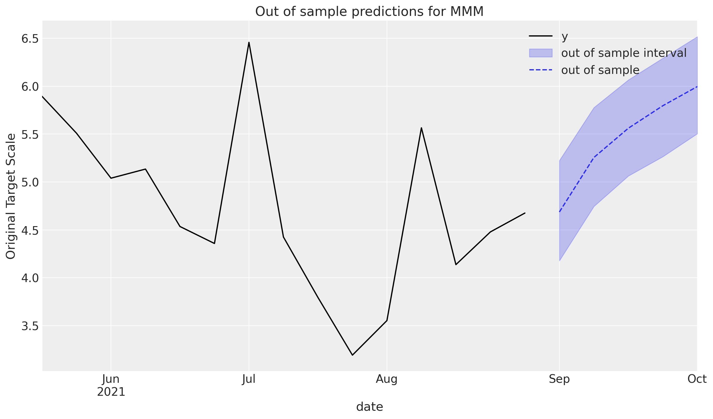
9. Out of Sample Predictions#

Out of sample predictions are can be done with the predict and posterior_predictivemethods. These include

sample_posterior_predictive : Get the full posterior predictive distribution
predict: Get the mean of the posterior predictive distribution

These methods take new data, X_pred, and some additional kwargs for new predictions. Namely,

include_last_observations : boolean flag in order to carry adstock effects from last observations in the training dataset

The new data needs to have all the features that are specified in the model. There is no need to worry about:

input scaling of channel spends or control features
creating fourier transformations on the date_column
inverse scaling back to target domain

That will be done automatically!

last_date = X["date_week"].max()

# New dates starting from last in dataset
n_new = 5
new_dates = pd.date_range(start=last_date, periods=1 + n_new, freq="W-MON")[1:]

X_out_of_sample = pd.DataFrame(
    {
        "date_week": new_dates,
    }
)

# Same channel spends as last day
X_out_of_sample["x1"] = X["x1"].iloc[-1]
X_out_of_sample["x2"] = X["x2"].iloc[-1]

# Other features
X_out_of_sample["event_1"] = 0
X_out_of_sample["event_2"] = 0

X_out_of_sample["t"] = range(len(X), len(X) + n_new)

X_out_of_sample

	date_week	x1	t
0	2021-09-06	0.438857	179
1	2021-09-13	0.438857	180
2	2021-09-20	0.438857	181
3	2021-09-27	0.438857	182
4	2021-10-04	0.438857	183

Call the desired method to get the new samples! The new coordinates will be from the new dates

NOTE: If the method is being called multiple times, set the extend_idata argument to False in order to not overwrite the observed_data in the InferenceData

The new predictions are transformed back to the original scale of the target by default. That can be seen below:

def plot_in_sample(X, y, ax, n_points: int = 15):
    (
        y.to_frame()
        .set_index(X["date_week"])
        .iloc[-n_points:]
        .plot(ax=ax, color="black", label="actuals")
    )


def plot_out_of_sample(X_out_of_sample, y_out_of_sample, ax, color, label):
    y_out_of_sample_groupby = y_out_of_sample["y"].to_series().groupby("date")

    lower, upper = quantiles = [0.025, 0.975]
    conf = y_out_of_sample_groupby.quantile(quantiles).unstack()
    ax.fill_between(
        X_out_of_sample["date_week"].dt.to_pydatetime(),
        conf[lower],
        conf[upper],
        alpha=0.25,
        color=color,
        label=f"{label} interval",
    )

    mean = y_out_of_sample_groupby.mean()
    mean.plot(ax=ax, label=label, color=color, linestyle="--")
    ax.set(ylabel="Original Target Scale", title="Out of sample predictions for MMM")

    return ax


_, ax = plt.subplots()
plot_in_sample(X, y, ax=ax)
plot_out_of_sample(
    X_out_of_sample, y_out_of_sample, ax=ax, label="out of sample", color="C0"
)
ax.legend();

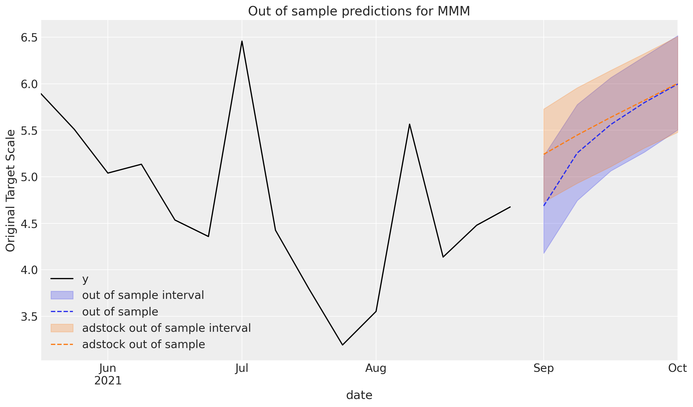
../../_images/77aca84665c287164846ac63ddc37f814ba54407a5ec5ee3f2f9bc906ddfe5e4.png

If the out of sample data is being extended from the original predictions, consider setting the include_last_observations to True in order to carry over the effects from the last channel spends in the training set.

The predictions are higher since the channel contributions the final spends still have an impact that eventually subside.

y_out_of_sample_with_adstock = mmm.sample_posterior_predictive(
    X_pred=X_out_of_sample, extend_idata=False, include_last_observations=True
)

Sampling: [y]

_, ax = plt.subplots()
plot_in_sample(X, y, ax=ax)
plot_out_of_sample(
    X_out_of_sample, y_out_of_sample, ax=ax, label="out of sample", color="C0"
)
plot_out_of_sample(
    X_out_of_sample,
    y_out_of_sample_with_adstock,
    ax=ax,
    label="adstock out of sample",
    color="C1",
)
ax.legend();

../../_images/b32907ddb493eddf7bff96465b9630a3f214b71ec893de0087aab2bf25e695a4.png

%load_ext watermark
%watermark -n -u -v -iv -w -p pytensor

Last updated: Fri Apr 12 2024

Python implementation: CPython
Python version       : 3.10.14
IPython version      : 8.22.2

pytensor: 2.20.0

seaborn   : 0.13.2
numpy     : 1.26.4
matplotlib: 3.8.3
arviz     : 0.17.1
pandas    : 2.2.1
pymc      : 5.13.0

Watermark: 2.4.3