Pareto/NBD Model#
The Pareto/Negative-Binomial Distribution model was the first Buy-Till-You-Die (BTYD) model for estimating non-contractual customer activity over a continuous time period. First introduced by Schmittlein, et. al. in 1987 and developed further by Bruce Hardie and Peter Fader, it is frequently used as a benchmark in CLV research due to its robust performance and wide range of functionality. For detailed derivations of this model please refer to “A Note on Deriving the Pareto/NBD Model and Related Expressions.”
In this notebook we will use Bayesian inference to fit a Pareto/NBD model in PyMC-Marketing. We will also demonstrate the predictive functionality of this model, along with an example for time-invariant covariates.
Setup Notebook#
import arviz as az
import matplotlib.pyplot as plt
import numpy as np
import pandas as pd
import pymc as pm
import seaborn as sb
import xarray as xr
from fastprogress.fastprogress import progress_bar
from pymc_extras.prior import Prior

from pymc_marketing import clv

# Plotting configuration
az.style.use("arviz-darkgrid")
plt.rcParams["figure.figsize"] = [12, 7]
plt.rcParams["figure.dpi"] = 100
plt.rcParams["figure.facecolor"] = "white"

%load_ext autoreload
%autoreload 2
%config InlineBackend.figure_format = "retina"
Load Data#
In this notebook we will be using the CDNOW sample dataset, a popular benchmarking dataset in CLV and BTYD modeling research. Refer here for more information about the dataset.
url_cdnow = "https://raw.githubusercontent.com/pymc-labs/pymc-marketing/main/data/cdnow_transactions.csv"

raw_data = pd.read_csv(url_cdnow)

raw_data.info()
raw_data.head()
<class 'pandas.core.frame.DataFrame'>
RangeIndex: 6919 entries, 0 to 6918
Data columns (total 5 columns):
 #   Column      Non-Null Count  Dtype
---  ------      --------------  -----
 0   _id         6919 non-null   int64
 1   id          6919 non-null   int64
 2   date        6919 non-null   int64
 3   cds_bought  6919 non-null   int64
 4   spent       6919 non-null   float64
dtypes: float64(1), int64(4)
memory usage: 270.4 KB
| _id | id | date | cds_bought | spent | |
|---|---|---|---|---|---|
| 0 | 4 | 1 | 19970101 | 2 | 29.33 |
| 1 | 4 | 1 | 19970118 | 2 | 29.73 |
| 2 | 4 | 1 | 19970802 | 1 | 14.96 |
| 3 | 4 | 1 | 19971212 | 2 | 26.48 |
| 4 | 21 | 2 | 19970101 | 3 | 63.34 |
The only requirements for modeling spending behaviour with ParetoNBDModel are a customer identifier column, and a datetime column for each purchase. The number of CDs purchased and money spent per transaction could also be useful covariates, so we’ll keep them in mind for later.
It is common for customer transaction databases to also contain returns, discount values, etc., so let’s do a quick validation check:
raw_data.describe()
| _id | id | date | cds_bought | spent | |
|---|---|---|---|---|---|
| count | 6919.000000 | 6919.000000 | 6.919000e+03 | 6919.000000 | 6919.000000 |
| mean | 11682.515826 | 1175.724816 | 1.997217e+07 | 2.381703 | 35.278500 |
| std | 6833.386793 | 679.426450 | 3.744182e+03 | 2.218380 | 34.074377 |
| min | 4.000000 | 1.000000 | 1.997010e+07 | 1.000000 | 0.000000 |
| 25% | 5525.000000 | 570.500000 | 1.997022e+07 | 1.000000 | 14.490000 |
| 50% | 11749.000000 | 1193.000000 | 1.997042e+07 | 2.000000 | 25.990000 |
| 75% | 17717.000000 | 1766.000000 | 1.997103e+07 | 3.000000 | 42.970000 |
| max | 23569.000000 | 2357.000000 | 1.998063e+07 | 40.000000 | 506.970000 |
Note there were some transactions with spend values of 0! Perhaps these were returns or promotional giveaways. Instances such as this are not true purchasing activities, and should be excluded from modeling.
raw_data = raw_data[raw_data["spent"] > 0]
Use the rfm_summary utility to aggregate data for modeling:
rfm_data = clv.rfm_summary(
    raw_data,
    customer_id_col="id",
    datetime_col="date",
    datetime_format="%Y%m%d",
    time_unit="W",
)

rfm_data.info()
rfm_data.head()
<class 'pandas.core.frame.DataFrame'>
RangeIndex: 2349 entries, 0 to 2348
Data columns (total 4 columns):
 #   Column       Non-Null Count  Dtype
---  ------       --------------  -----
 0   customer_id  2349 non-null   int64
 1   frequency    2349 non-null   float64
 2   recency      2349 non-null   float64
 3   T            2349 non-null   float64
dtypes: float64(3), int64(1)
memory usage: 73.5 KB
| customer_id | frequency | recency | T | |
|---|---|---|---|---|
| 0 | 1 | 3.0 | 49.0 | 78.0 |
| 1 | 2 | 1.0 | 2.0 | 78.0 |
| 2 | 3 | 0.0 | 0.0 | 78.0 |
| 3 | 4 | 0.0 | 0.0 | 78.0 |
| 4 | 5 | 0.0 | 0.0 | 78.0 |
Recall the data aggregation definitions from the CLV Quickstart:
customer_idis an index of a unique identifiers for each customer.frequencyis the number of repeat purchases that a customer has made (i.e., total number of purchases minus one).recencyindicates the time period when a customer made their most recent purchase. If a customer has only made 1 purchase, recency is 0.Tis a customer’s “age”, or the number of time periods since their first purchase.
Model Definition#
The Pareto/NBD model is based on the following assumptions for each customer:
Customers are active for an unobserved period of time, then become permanently inactive.
Purchasing Process#
While active, the the number of transactions made by a customer follows a Poisson process with transaction rate \(\lambda\):
\[P(X(t)=x|\lambda) = \frac{(\lambda t)^{x}e^{-\lambda t}}{x!}, x=0,1,2,...\]This is equivalent to assuming time between transactions is exponentially distributed with transaction rate \(\lambda\):
\[f(t_{j}-t_{j-1}| \lambda) = \lambda e^{-\lambda (t_{j} - t_{j - 1})}, \quad t_{j} \geq t_{j - 1} \geq 0\]Where \(t\) is the time period of the \(j\)th purchase.
Heterogeneity in \(\lambda\) follows a Gamma distribution with shape parameter \(r\) and scale parameter \(\alpha\):
\[g(\lambda|r, \alpha) = \frac{\alpha^{r}\lambda^{r - 1}e^{-\lambda \alpha}}{\Gamma(r)}\]
Dropout Process#
The duration of a customer’s unobserved active lifetime is exponentially distributed with dropout rate \(\mu\).
Heterogeneity in \(\mu\) also follows a Gamma distribution with shape parameter \(s\) and scale parameter \(\beta\):
\[g(\mu|s, \beta) = \frac{\beta^{s}\mu^{s - 1}e^{-\mu \beta}}{\Gamma(s)}\]Transaction rate \(\lambda\) and time until dropout \(\mu\) vary independently for each customer.
If we take the expectation across the distributions of \(\lambda\) and \(\mu\), we can derive a likelihood function to estimate parameters \(r\), \(\alpha\), \(s\), and \(\beta\) across the customer population. For more details on the ParetoNBD likelihood please refer to the docs.
Model Fitting#
The Bayesian equivalent of Maximum Likelihood Estimation (MLE) is Maximum a Posteriori (MAP), where scalar values for fitted parameters are regularized with priors during estimation.
A “Flat” prior indicates the user is agnostic, holding no prior beliefs or assumptions about the data. \(r\), \(\alpha\), \(s\), and \(\beta\) must also be positive values, so let’s configure our Bayesian ParetoNBDModel with HalfFlat priors:
flat_config = {
    "r": Prior("HalfFlat"),
    "alpha": Prior("HalfFlat"),
    "s": Prior("HalfFlat"),
    "beta": Prior("HalfFlat"),
}

pnbd_pymc = clv.ParetoNBDModel(model_config=flat_config)
Build the model to view the choice of Priors used for modeling:
pnbd_pymc.build_model(data=rfm_data)  # optional step
pnbd_pymc
Pareto/NBD
            alpha ~ HalfFlat()
             beta ~ HalfFlat()
                r ~ HalfFlat()
                s ~ HalfFlat()
recency_frequency ~ ParetoNBD(r, alpha, s, beta, <constant>)
Note it is not necessary to build a model prior to modeling.
Now let’s fit our ParetoNBDModel with MAP.
idata_map = pnbd_pymc.fit(method="map")
For MAP fitting pymc-marketing uses the L-BGFS-B optimizer from scipy.optimize, a faster and more stable alternative to Nelder-Mead.
flat_fit = pnbd_pymc.fit_summary()
print(flat_fit)
alpha    15.644
beta     13.796
r         0.614
s         0.447
Name: value, dtype: float64
The CDNOW sample we’re working with is quite small and comprises only 10% of the total CDNOW dataset, so it’s quite likely these estimates are overfitting if we attempt to run predictions on the full dataset.
With prior distributions, we can inform model fitting with our own subjective domain knowledge, and even improve the speed of model fits. The default prior configuration for ParetoNBDModel works well for a variety of use cases:
pnbd_map = clv.ParetoNBDModel()
pnbd_map.build_model(data=rfm_data)  # required for prior predictive checks
pnbd_map
Pareto/NBD
            alpha ~ Weibull(2, 10)
             beta ~ Weibull(2, 10)
                r ~ Weibull(2, 1)
                s ~ Weibull(2, 1)
recency_frequency ~ ParetoNBD(r, alpha, s, beta, <constant>)
Prior and Posterior Predictive Checks#
PPCs allow us to check the efficacy of our priors, and the peformance of the fitted posteriors. PPCs aren’t usually an option with MAP fitted models, but here we’re actually sampling from the latent \(\lambda\) and \(\mu\) Gamma distributions, so PPCs are possible for ParetoNBDModel regardless of the fit method!
Let’s see how the model performs in a prior predictive check, where we sample from the default priors before fitting the model:
with pnbd_map.model:
    prior_idata = pm.sample_prior_predictive(random_seed=45, draws=1)

obs_freq = prior_idata.observed_data["recency_frequency"].sel(obs_var="frequency")
ppc_freq = prior_idata.prior_predictive["recency_frequency"].sel(obs_var="frequency")[
    0
][0]

# PPC histogram plot
clv.plot_expected_purchases_ppc(pnbd_map, ppc="prior");
Sampling: [alpha, beta, r, recency_frequency, s]
Sampling: [alpha, beta, r, recency_frequency, s]
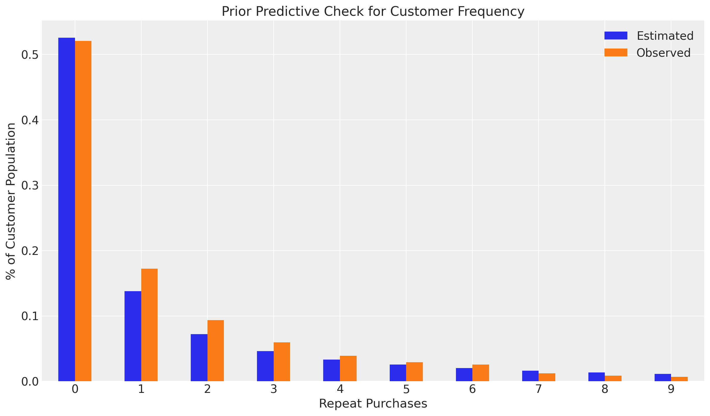
Here the ParetoNBDModel is simulating customer purchases from the prior distributions to compare against the obseved data. The default priors look reasonable for non-repeat customers, but do not model repeat customers well.
Let’s fit our model and run a posterior predictive check for comparison:
pnbd_map.fit()
map_fit = pnbd_map.fit_summary()  # save for plotting later

obs_freq = pnbd_map.idata.observed_data["recency_frequency"].sel(obs_var="frequency")
ppc_freq = pnbd_map.distribution_new_customer_recency_frequency(
    rfm_data,
    random_seed=42,
).sel(chain=0, draw=0, obs_var="frequency")

# PPC histogram plot
clv.plot_expected_purchases_ppc(pnbd_map, ppc="posterior");
Sampling: [recency_frequency]
Sampling: [recency_frequency]

Our fitted model is able to reliably simulate customer behavior!
Full Bayesian Inference#
MAP fits estimate only scalar values for \(r\), \(\alpha\), \(s\), and \(\beta\), but with full Bayesian sampling we can infer the posterior probability distributions for these parameters, illustrating uncertainty in our estimates as well as enabling prediction intervals.
NUTS is the default sampler in pymc-marketing, which samples from the posterior by exploring the gradients of the probability space. However, NUTS sampling with ParetoNBDModel can be quite slow due to the complexity of the likelihood expression. In fact, the mathematical complexity of this model is what motivated the development of the BetaGeoModel in 2005. The BG/NBD model makes some simplifying assumptions and sacrifices functionality in customer dropout estimation for better computational performance.
To save time and computational costs, it is recommended to use the gradient-free DEMetropolisZ sampler. This often requires more samples during fitting, so if any rhat statistic warnings are encountered, increase the size of the tune and draw parameters until the warning no longer appears.
pnbd_full = clv.ParetoNBDModel()
pnbd_full.fit(
    data=rfm_data,
    method="demz",
    draws=3000,
    tune=2500,
    idata_kwargs={"log_likelihood": True},
)
Multiprocess sampling (4 chains in 4 jobs)
DEMetropolisZ: [alpha, beta, r, s]
Sampling 4 chains for 2_500 tune and 3_000 draw iterations (10_000 + 12_000 draws total) took 6 seconds.
-
<xarray.Dataset> Size: 408kB Dimensions: (chain: 4, draw: 3000) Coordinates: * chain (chain) int64 32B 0 1 2 3 * draw (draw) int64 24kB 0 1 2 3 4 5 6 ... 2994 2995 2996 2997 2998 2999 Data variables: alpha (chain, draw) float64 96kB 15.45 15.45 15.45 ... 15.71 15.71 17.46 beta (chain, draw) float64 96kB 14.67 14.67 14.67 ... 14.4 14.4 10.09 r (chain, draw) float64 96kB 0.6189 0.6189 0.6189 ... 0.6553 0.7206 s (chain, draw) float64 96kB 0.4866 0.4866 0.4866 ... 0.4811 0.3935 Attributes: created_at: 2024-12-13T07:35:40.505430+00:00 arviz_version: 0.18.0 inference_library: pymc inference_library_version: 5.15.1 sampling_time: 6.140834093093872 tuning_steps: 2500 -
<xarray.Dataset> Size: 226MB Dimensions: (chain: 4, draw: 3000, customer_id: 2349) Coordinates: * chain (chain) int64 32B 0 1 2 3 * draw (draw) int64 24kB 0 1 2 3 4 ... 2995 2996 2997 2998 2999 * customer_id (customer_id) int64 19kB 1 2 3 4 ... 2354 2355 2356 2357 Data variables: recency_frequency (chain, draw, customer_id) float64 226MB -14.3 ... -0.... Attributes: created_at: 2024-12-13T07:35:46.109420+00:00 arviz_version: 0.18.0 inference_library: pymc inference_library_version: 5.15.1 -
<xarray.Dataset> Size: 324kB Dimensions: (chain: 4, draw: 3000) Coordinates: * chain (chain) int64 32B 0 1 2 3 * draw (draw) int64 24kB 0 1 2 3 4 5 6 ... 2994 2995 2996 2997 2998 2999 Data variables: accept (chain, draw) float64 96kB 0.003792 0.02374 ... 3.073e-05 0.2678 accepted (chain, draw) bool 12kB False False False True ... True False True lambda (chain, draw) float64 96kB 0.8415 0.8415 0.8415 ... 0.8415 0.8415 scaling (chain, draw) float64 96kB 0.0001501 0.0001501 ... 0.0001337 Attributes: created_at: 2024-12-13T07:35:40.508144+00:00 arviz_version: 0.18.0 inference_library: pymc inference_library_version: 5.15.1 sampling_time: 6.140834093093872 tuning_steps: 2500 -
<xarray.Dataset> Size: 56kB Dimensions: (customer_id: 2349, obs_var: 2) Coordinates: * customer_id (customer_id) int64 19kB 1 2 3 4 ... 2354 2355 2356 2357 * obs_var (obs_var) <U9 72B 'recency' 'frequency' Data variables: recency_frequency (customer_id, obs_var) float64 38kB 49.0 3.0 ... 0.0 0.0 Attributes: created_at: 2024-12-13T07:35:40.509416+00:00 arviz_version: 0.18.0 inference_library: pymc inference_library_version: 5.15.1 -
<xarray.Dataset> Size: 94kB
Dimensions:      (index: 2349)
Coordinates:
  * index        (index) int64 19kB 0 1 2 3 4 5 ... 2344 2345 2346 2347 2348
Data variables:
    customer_id  (index) int64 19kB 1 2 3 4 5 6 ... 2353 2354 2355 2356 2357
    frequency    (index) float64 19kB 3.0 1.0 0.0 0.0 0.0 ... 5.0 1.0 6.0 0.0
    recency      (index) float64 19kB 49.0 2.0 0.0 0.0 ... 24.0 44.0 62.0 0.0
    T            (index) float64 19kB 78.0 78.0 78.0 78.0 ... 66.0 66.0 66.0
pnbd_full.fit_summary()
| mean | sd | hdi_3% | hdi_97% | mcse_mean | mcse_sd | ess_bulk | ess_tail | r_hat | |
|---|---|---|---|---|---|---|---|---|---|
| alpha | 15.769 | 1.114 | 13.717 | 17.876 | 0.038 | 0.027 | 882.0 | 1152.0 | 1.01 |
| beta | 12.565 | 3.630 | 6.598 | 19.738 | 0.124 | 0.088 | 821.0 | 1072.0 | 1.00 |
| r | 0.627 | 0.049 | 0.540 | 0.721 | 0.002 | 0.001 | 845.0 | 1100.0 | 1.00 |
| s | 0.428 | 0.060 | 0.321 | 0.541 | 0.002 | 0.001 | 838.0 | 1212.0 | 1.00 |
Use thin_fit_result if the large number of draws are causing computational issues. Keeping every second sample will reduce the number of draws by half:
pnbd_full.thin_fit_result(keep_every=2).idata
-
<xarray.Dataset> Size: 204kB Dimensions: (chain: 4, draw: 1500) Coordinates: * chain (chain) int64 32B 0 1 2 3 * draw (draw) int64 12kB 0 2 4 6 8 10 12 ... 2988 2990 2992 2994 2996 2998 Data variables: alpha (chain, draw) float64 48kB 15.45 15.45 17.23 ... 14.82 14.82 15.71 beta (chain, draw) float64 48kB 14.67 14.67 15.43 ... 14.21 14.21 14.4 r (chain, draw) float64 48kB 0.6189 0.6189 0.6611 ... 0.5998 0.6553 s (chain, draw) float64 48kB 0.4866 0.4866 0.502 ... 0.4529 0.4811 Attributes: created_at: 2024-12-13T07:35:40.505430+00:00 arviz_version: 0.18.0 inference_library: pymc inference_library_version: 5.15.1 sampling_time: 6.140834093093872 tuning_steps: 2500 -
<xarray.Dataset> Size: 113MB Dimensions: (chain: 4, draw: 1500, customer_id: 2349) Coordinates: * chain (chain) int64 32B 0 1 2 3 * draw (draw) int64 12kB 0 2 4 6 8 ... 2990 2992 2994 2996 2998 * customer_id (customer_id) int64 19kB 1 2 3 4 ... 2354 2355 2356 2357 Data variables: recency_frequency (chain, draw, customer_id) float64 113MB -14.3 ... -0.654 Attributes: created_at: 2024-12-13T07:35:46.109420+00:00 arviz_version: 0.18.0 inference_library: pymc inference_library_version: 5.15.1 -
<xarray.Dataset> Size: 162kB Dimensions: (chain: 4, draw: 1500) Coordinates: * chain (chain) int64 32B 0 1 2 3 * draw (draw) int64 12kB 0 2 4 6 8 10 ... 2988 2990 2992 2994 2996 2998 Data variables: accept (chain, draw) float64 48kB 0.003792 1.95e-06 ... 0.1581 3.073e-05 accepted (chain, draw) bool 6kB False False False ... False False False lambda (chain, draw) float64 48kB 0.8415 0.8415 0.8415 ... 0.8415 0.8415 scaling (chain, draw) float64 48kB 0.0001501 0.0001501 ... 0.0001337 Attributes: created_at: 2024-12-13T07:35:40.508144+00:00 arviz_version: 0.18.0 inference_library: pymc inference_library_version: 5.15.1 sampling_time: 6.140834093093872 tuning_steps: 2500 -
<xarray.Dataset> Size: 56kB Dimensions: (customer_id: 2349, obs_var: 2) Coordinates: * customer_id (customer_id) int64 19kB 1 2 3 4 ... 2354 2355 2356 2357 * obs_var (obs_var) <U9 72B 'recency' 'frequency' Data variables: recency_frequency (customer_id, obs_var) float64 38kB 49.0 3.0 ... 0.0 0.0 Attributes: created_at: 2024-12-13T07:35:40.509416+00:00 arviz_version: 0.18.0 inference_library: pymc inference_library_version: 5.15.1 -
<xarray.Dataset> Size: 94kB
Dimensions:      (index: 2349)
Coordinates:
  * index        (index) int64 19kB 0 1 2 3 4 5 ... 2344 2345 2346 2347 2348
Data variables:
    customer_id  (index) int64 19kB 1 2 3 4 5 6 ... 2353 2354 2355 2356 2357
    frequency    (index) float64 19kB 3.0 1.0 0.0 0.0 0.0 ... 5.0 1.0 6.0 0.0
    recency      (index) float64 19kB 49.0 2.0 0.0 0.0 ... 24.0 44.0 62.0 0.0
    T            (index) float64 19kB 78.0 78.0 78.0 78.0 ... 66.0 66.0 66.0
axes = az.plot_trace(
    data=pnbd_full.idata,
    compact=True,
    kind="rank_bars",
    backend_kwargs={"figsize": (12, 7), "layout": "constrained"},
)
plt.gcf().suptitle("Pareto/NBD Model Trace", fontsize=18, fontweight="bold");
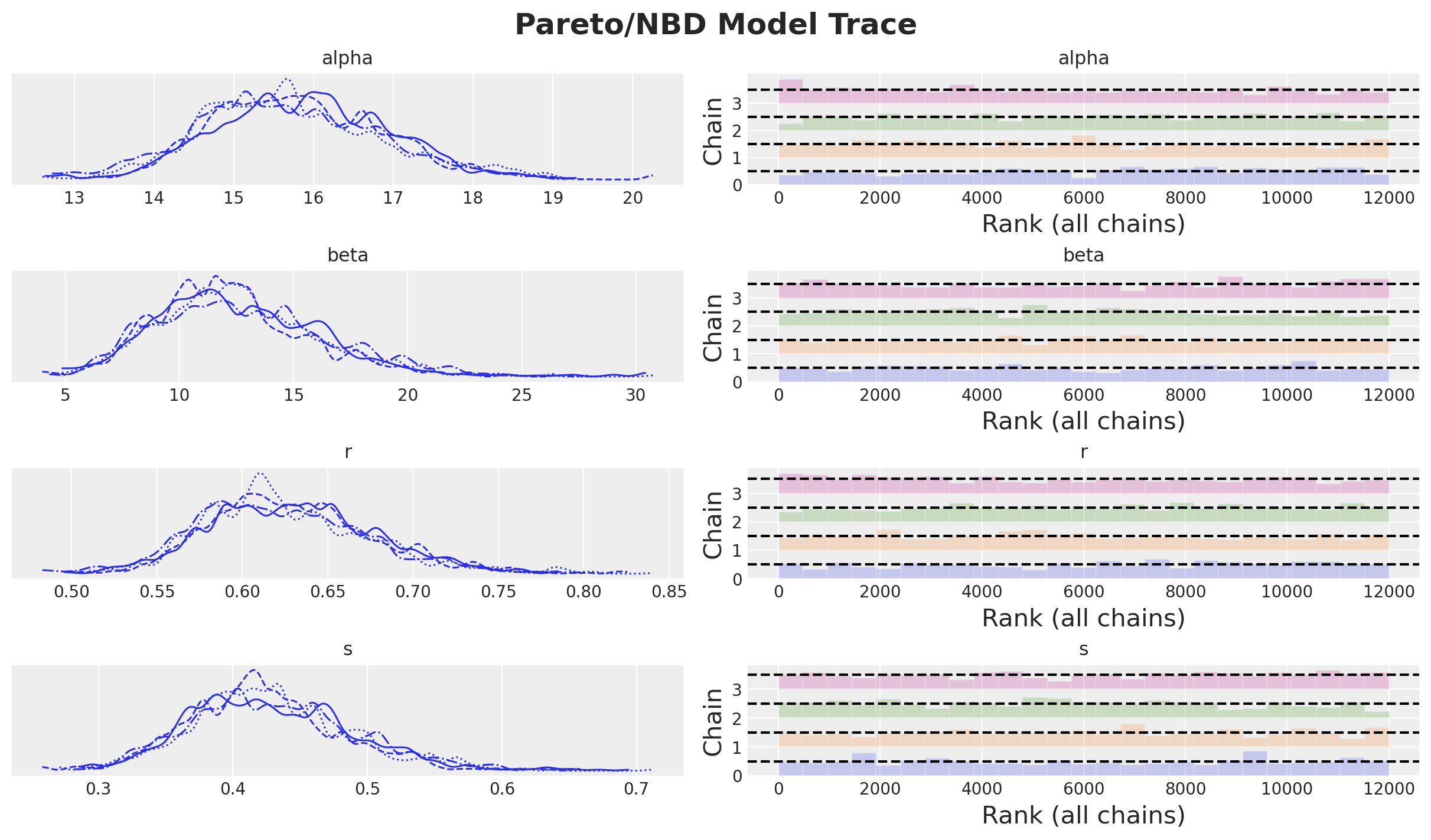
pnbd_full.idata
-
<xarray.Dataset> Size: 408kB Dimensions: (chain: 4, draw: 3000) Coordinates: * chain (chain) int64 32B 0 1 2 3 * draw (draw) int64 24kB 0 1 2 3 4 5 6 ... 2994 2995 2996 2997 2998 2999 Data variables: alpha (chain, draw) float64 96kB 16.12 16.12 16.12 ... 16.76 16.76 16.76 beta (chain, draw) float64 96kB 16.98 16.98 16.98 ... 8.639 8.639 8.639 r (chain, draw) float64 96kB 0.635 0.635 0.635 ... 0.6551 0.6551 s (chain, draw) float64 96kB 0.5287 0.5287 0.5287 ... 0.3744 0.3744 Attributes: created_at: 2024-11-23T22:32:50.642976+00:00 arviz_version: 0.18.0 inference_library: pymc inference_library_version: 5.15.1 sampling_time: 6.095298767089844 tuning_steps: 2500 -
<xarray.Dataset> Size: 226MB Dimensions: (chain: 4, draw: 3000, customer_id: 2349) Coordinates: * chain (chain) int64 32B 0 1 2 3 * draw (draw) int64 24kB 0 1 2 3 4 ... 2995 2996 2997 2998 2999 * customer_id (customer_id) int64 19kB 1 2 3 4 ... 2354 2355 2356 2357 Data variables: recency_frequency (chain, draw, customer_id) float64 226MB -14.28 ... -0... Attributes: created_at: 2024-11-23T22:32:56.529120+00:00 arviz_version: 0.18.0 inference_library: pymc inference_library_version: 5.15.1 -
<xarray.Dataset> Size: 324kB Dimensions: (chain: 4, draw: 3000) Coordinates: * chain (chain) int64 32B 0 1 2 3 * draw (draw) int64 24kB 0 1 2 3 4 5 6 ... 2994 2995 2996 2997 2998 2999 Data variables: accept (chain, draw) float64 96kB 0.4747 0.0004368 ... 0.007007 0.4167 accepted (chain, draw) bool 12kB False False False ... False False False lambda (chain, draw) float64 96kB 0.8415 0.8415 0.8415 ... 0.8415 0.8415 scaling (chain, draw) float64 96kB 0.0002542 0.0002542 ... 0.0002288 Attributes: created_at: 2024-11-23T22:32:50.645501+00:00 arviz_version: 0.18.0 inference_library: pymc inference_library_version: 5.15.1 sampling_time: 6.095298767089844 tuning_steps: 2500 -
<xarray.Dataset> Size: 56kB
Dimensions:            (customer_id: 2349, obs_var: 2)
Coordinates:
  * customer_id        (customer_id) int64 19kB 1 2 3 4 ... 2354 2355 2356 2357
  * obs_var            (obs_var) <U9 72B 'recency' 'frequency'
Data variables:
    recency_frequency  (customer_id, obs_var) float64 38kB 49.0 3.0 ... 0.0 0.0
Attributes:
    created_at:                 2024-11-23T22:32:50.646870+00:00
    arviz_version:              0.18.0
    inference_library:          pymc
    inference_library_version:  5.15.1
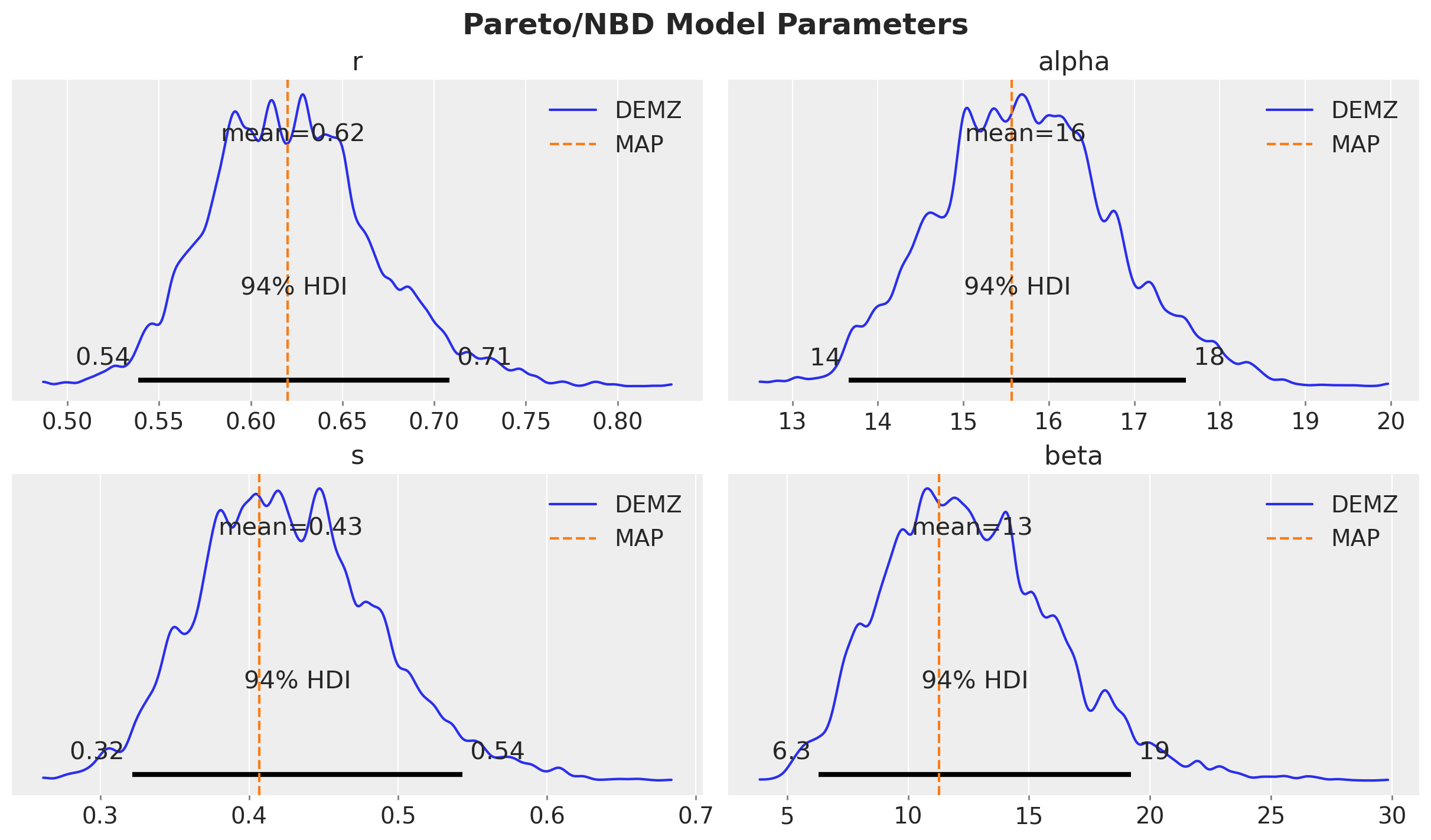
Let’s see how the DEMZ posteriors compare to the MAP estimations:
_, axes = plt.subplots(
    nrows=2, ncols=2, figsize=(12, 7), sharex=False, sharey=False, layout="constrained"
)

axes = axes.flatten()

for i, var_name in enumerate(["r", "alpha", "s", "beta"]):
    ax = axes[i]
    az.plot_posterior(
        pnbd_full.idata.posterior[var_name].values.flatten(),
        color="C0",
        point_estimate="mean",
        ax=ax,
        label="DEMZ",
    )
    ax.axvline(x=map_fit[var_name], color="C1", linestyle="--", label="MAP")
    ax.legend(loc="upper right")
    ax.set_title(var_name)

plt.gcf().suptitle("Pareto/NBD Model Parameters", fontsize=18, fontweight="bold");
After fitting, models can be persisted with pnbd_pymc.save("pnbd.nc") and pnbd_pymc.load("pnbd.nc").
Predictive Methods#
The Pareto/NBD model supports a variety of predictive methods:
expected_purchasesexpected_probability_aliveexpected_purchases_new_customerexpected_purchase_probability
Let’s take a small sample of users:
example_customer_ids = [1, 5, 10, 18, 46, 1413]

rfm_sample = rfm_data.query("customer_id.isin(@example_customer_ids)")

rfm_sample.sort_values(by="frequency")
| customer_id | frequency | recency | T | |
|---|---|---|---|---|
| 4 | 5 | 0.0 | 0.0 | 78.0 |
| 9 | 10 | 0.0 | 0.0 | 78.0 |
| 17 | 18 | 1.0 | 5.0 | 78.0 |
| 0 | 1 | 3.0 | 49.0 | 78.0 |
| 1405 | 1413 | 19.0 | 54.0 | 71.0 |
| 45 | 46 | 21.0 | 73.0 | 78.0 |
Observe customers 5 & 10 are non-repeat buyers, whereas 1413 and 46 are frequent buyers.
Expected Number of Purchases#
Let’s plot each customer’s expected number of purchases over the next \(90\) time periods:
time_periods = 90

expected_purchases_over_time = xr.concat(
    objs=[
        pnbd_full.expected_purchases(
            data=rfm_sample,
            future_t=t,
        )
        for t in progress_bar(range(time_periods))
    ],
    dim="t",
).transpose(..., "t")
_, axes = plt.subplots(
    nrows=len(example_customer_ids),
    ncols=1,
    figsize=(12, 14),
    sharex=True,
    sharey=True,
    layout="constrained",
)

axes = axes.flatten()

for i, customer_id in enumerate(example_customer_ids):
    ax = axes[i]
    customer_expected_purchases = expected_purchases_over_time.sel(
        customer_id=customer_id
    )
    az.plot_hdi(
        range(time_periods),
        customer_expected_purchases,
        hdi_prob=0.94,
        color="C0",
        fill_kwargs={"alpha": 0.3, "label": "$94 \\%$ HDI"},
        ax=ax,
    )
    az.plot_hdi(
        range(time_periods),
        customer_expected_purchases,
        hdi_prob=0.5,
        color="C0",
        fill_kwargs={"alpha": 0.5, "label": "$50 \\%$ HDI"},
        ax=ax,
    )
    ax.plot(
        range(time_periods),
        customer_expected_purchases.mean(dim=("chain", "draw")),
        color="C0",
        label="posterior mean",
    )
    ax.legend(loc="upper left")
    ax.set(title=f"Customer {customer_id}", xlabel="t", ylabel="# of purchases")

axes[-1].set(xlabel="t")
plt.gcf().suptitle("Expected Number of Purchases", fontsize=18, fontweight="bold");
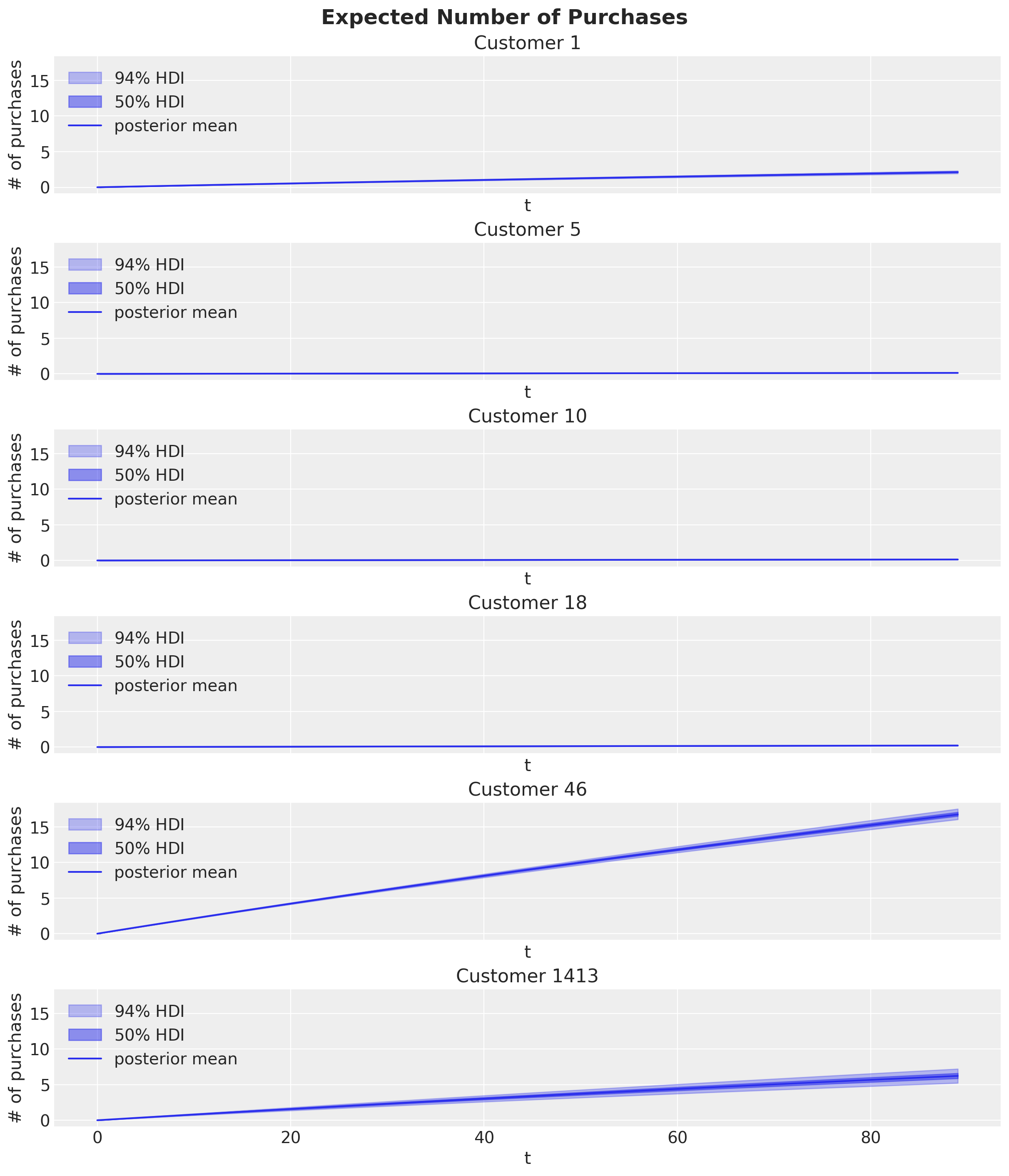
Note the HDI prediction intervals are only available if the model is fit with full posteriors.
Observe the large number of purchases expected from the frequent buyers (Customers 46 and 1413) whereas little or no future activity is expected of the remaining customers.
Expected Probability Alive#
Let’s check the probability our customers are still alive and compare against the MAP results.
_, axes = plt.subplots(
    nrows=3,
    ncols=2,
    figsize=(12, 14),
    layout="constrained",
)

axes = axes.flatten()

for i, customer_id in enumerate(example_customer_ids):
    ax = axes[i]
    demz_alive = pnbd_full.expected_probability_alive(
        rfm_sample,
        future_t=0,
    ).sel(customer_id=customer_id)
    map_alive = pnbd_map.expected_probability_alive(rfm_sample, future_t=0).sel(
        customer_id=customer_id
    )

    az.plot_density(demz_alive, hdi_prob=1, colors="C1", shade=0.3, bw=0.005, ax=ax)
    ax.axvline(x=map_alive, color="C3", linestyle="--", label="MAP")
    ax.legend(loc="upper right")
    ax.set(
        title=f"Customer {customer_id}",
        xlabel="Probability Alive",
        ylabel="Posterior Density",
    )

plt.gcf().suptitle("Expected Probability Alive", fontsize=18, fontweight="bold");

Customer 1413 has a rather low alive probability despite being a frequent purchaser. This would be a good example of a customer to target with a special offer for retention.
These probabilities are estimated at time period 0, but we can also estimate the probabilities customers will still be active in the future. Let’s calculate the posterior densities 90 time periods from now and compare to the MAP at time period 0:
_, axes = plt.subplots(
    nrows=3,
    ncols=2,
    figsize=(12, 14),
    layout="constrained",
)

axes = axes.flatten()

for i, customer_id in enumerate(example_customer_ids):
    ax = axes[i]
    demz_alive = pnbd_full.expected_probability_alive(
        rfm_sample,
        future_t=90,
    ).sel(customer_id=customer_id)
    map_alive = pnbd_map.expected_probability_alive(rfm_sample, future_t=0).sel(
        customer_id=customer_id
    )

    az.plot_density(demz_alive, hdi_prob=1, colors="C1", shade=0.3, bw=0.005, ax=ax)
    ax.axvline(x=map_alive, color="C3", linestyle="--", label="MAP at Time 0")
    ax.legend(loc="upper left")
    ax.set(
        title=f"Customer {customer_id}",
        xlabel="Probability Alive",
        ylabel="Posterior Density at Time 90",
    )

plt.gcf().suptitle("Expected Probability Alive Delta", fontsize=18, fontweight="bold");

Pay attention to the x-axes for each customer - The probabilities barely changed for the non-repeat customers, but there is a significant delta for frequent buyers.
A good rule of thumb is that an alive probability of .25-.30 usually indicates an at-risk or inactive customer. Future projections can give additional insight into customer churn risk.
Probability of \(n\) Purchases over Time \(t\)#
Customer 46 is our best customer in this small sample set, and is expected to make at least \(15\) purchases over the next \(90\) time periods. What is the probability of this many purchases being made, and how will it change over time?
Let’s plot a heatmap to paint the full picture:
# create arrays of parameter combinations
n_purchases = np.repeat([0, 3, 6, 9, 12, 15], 6)
time_periods = np.tile([15, 30, 45, 60, 75, 90], 6)

expected_purchase_prob_heatmap = xr.concat(
    objs=[
        pnbd_map.expected_purchase_probability(
            rfm_sample,
            n_purchases=params[0],
            future_t=params[1],
        ).sel(customer_id=46)
        for params in zip(n_purchases, time_periods, strict=False)
    ],
    dim="customer_id",
).transpose(..., "customer_id")
heatmap_reshape = expected_purchase_prob_heatmap.values.reshape(6, 6)

sb.heatmap(heatmap_reshape, annot=True)

plt.xlabel("Time Periods")
plt.xticks(np.arange(6) + 0.5, [15, 30, 45, 60, 75, 90], rotation=0)
plt.ylabel("Number of Purchases")
plt.yticks(np.arange(6) + 0.5, [0, 3, 6, 9, 12, 15], rotation=0)
plt.gcf().suptitle(
    "Expected Purchase Probabilities for Customer 46", fontsize=18, fontweight="bold"
);
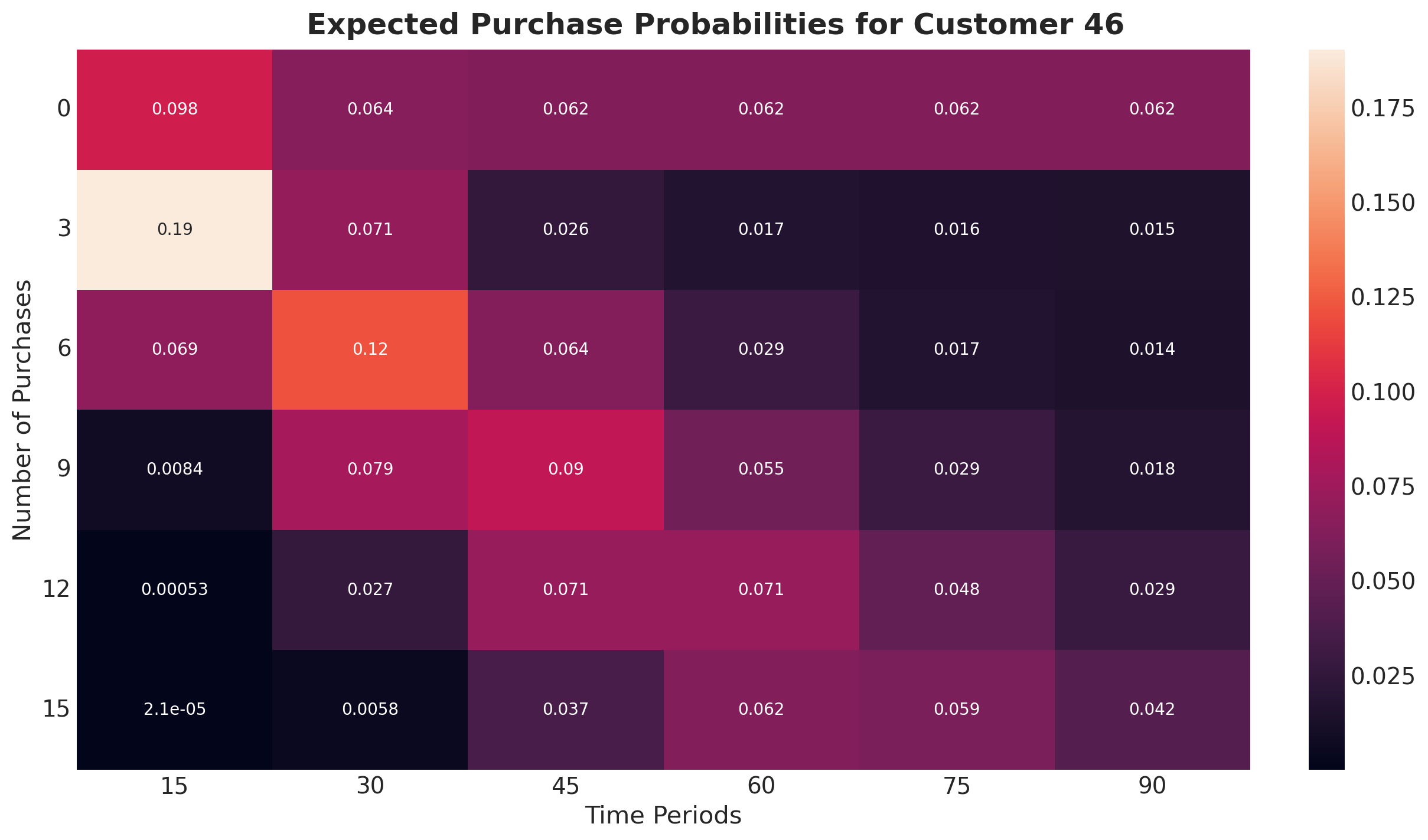
This heatmap highlights how Customer 46 is expected to make at least 15 purchases up to time period 90, but the odds of 15 purchases being made before time period 75 or even time period 60 are slightly higher. Also note these probabilities assume exact expectations (i.e., there’s a 6.2% chance of the 15th purchase being made precisely during time period 60.)
Expected Number of Purchases for New Customers#
So far we’ve only been running predictions for existing customers, but we can also estimate the expected number of transactions over time for a new customer:
expected_purchases_over_time_new_customer = xr.concat(
    objs=[
        pnbd_full.expected_purchases_new_customer(
            data=rfm_sample,
            t=t,
        ).sel(customer_id=1)  # customer_id is arbitrary here
        for t in range(90)
    ],
    dim="t",
).transpose(..., "t")


# plot results
ax = plt.axes()

az.plot_hdi(
    range(90),
    expected_purchases_over_time_new_customer,
    hdi_prob=0.94,
    color="C2",
    fill_kwargs={"alpha": 0.3, "label": "$94 \\%$ HDI"},
    ax=ax,
)
az.plot_hdi(
    range(90),
    expected_purchases_over_time_new_customer,
    hdi_prob=0.5,
    color="C2",
    fill_kwargs={"alpha": 0.5, "label": "$50 \\%$ HDI"},
    ax=ax,
)
ax.plot(
    range(90),
    expected_purchases_over_time_new_customer.mean(dim=("chain", "draw")),
    color="C2",
    label="posterior mean",
)
ax.legend(loc="upper left")
ax.set(
    title="Expected Number of Purchases by New Customers",
    ylabel="# of purchases",
    xlabel="t",
);

Let’s see how these estimates change when we add covariates to the model.
Time-Invariant Covariates#
Recall \(\alpha\), and \(\beta\) represent the scale parameters for the purchase and dropout rate distributions, respectively. To model for time-invariant covariates, we simply modify these parameters as follows:
Where \(\gamma_1\) and \(\gamma_2\) are coefficients capturing the impact of the covariates, and \(z_1\) and \(z_2\) the covariate arrays for each customer.
Let’s take a look at the covariates available in the raw data:
# aggregate raw data by customer id
covar_df = raw_data[["id", "cds_bought", "spent"]].groupby("id").mean().reset_index()

# plot covariate histograms
_, axes = plt.subplots(
    nrows=1,
    ncols=2,
    figsize=(10, 5),
    layout="constrained",
)

axes = axes.flatten()

covars = ["cds_bought", "spent"]
colors = ["C0", "C2"]

for ax in zip(axes, covars, colors, strict=False):
    ax[0].hist(
        x=covar_df[ax[1]],
        bins=5,
        color=ax[2],
    )
    ax[0].set(title=f"{ax[1]}", xlabel="value", ylabel="count")
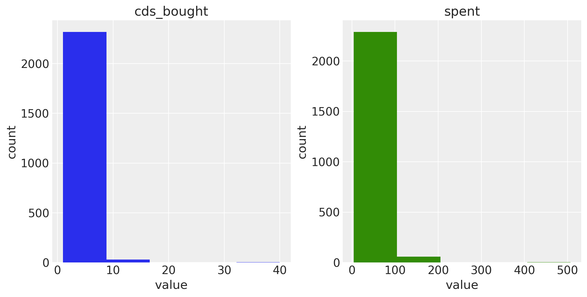
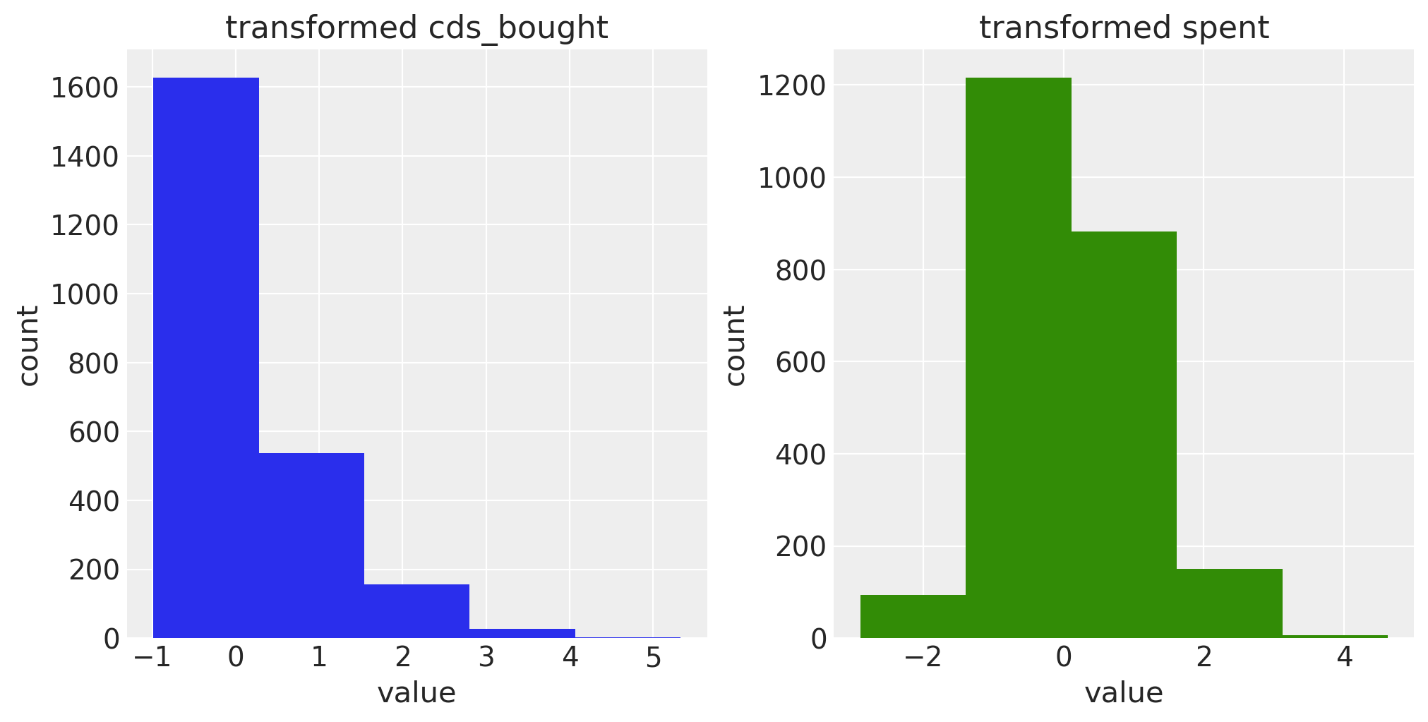
One-tailed distributions with large values like this will complicate model fitting, so let’s log and standardize our covariates:
for covar in ["cds_bought", "spent"]:
    covar_df[f"log_std_{covar}"] = np.log(covar_df[covar]).copy()
    covar_df[f"log_std_{covar}"] -= np.nanmean(covar_df[f"log_std_{covar}"])
    covar_df[f"log_std_{covar}"] /= np.nanstd(covar_df[f"log_std_{covar}"])
    covar_df[f"log_std_{covar}"] = covar_df[f"log_std_{covar}"].fillna(0)

_, axes = plt.subplots(
    nrows=1,
    ncols=2,
    figsize=(10, 5),
    layout="constrained",
)

axes = axes.flatten()

for ax in zip(axes, covars, colors, strict=False):
    ax[0].hist(
        x=covar_df[f"log_std_{ax[1]}"],
        bins=5,
        color=ax[2],
    )
    ax[0].set(title=f"transformed {ax[1]}", xlabel="value", ylabel="count")
To parametrize ParetoNBDModel with covariates, join the covariates to the existing RFM data and specify the column names in the model_config. Covariates for the purchase and dropout rates can be specified separately, enabling experimentation with various combinations to find what works best:
rfm_covar = rfm_data.merge(covar_df, left_on="customer_id", right_on="id", how="inner")

pnbd_covar = clv.ParetoNBDModel(
    model_config={
        "purchase_covariate_cols": ["log_std_cds_bought", "log_std_spent"],
        "dropout_covariate_cols": ["log_std_cds_bought", "log_std_spent"],
    },
)

pnbd_covar.build_model(rfm_covar)
pnbd_covar
Pareto/NBD
purchase_coefficient ~ Normal(0, 1)
         alpha_scale ~ Weibull(2, 10)
 dropout_coefficient ~ Normal(0, 1)
          beta_scale ~ Weibull(2, 10)
                   r ~ Weibull(2, 1)
                   s ~ Weibull(2, 1)
               alpha ~ Deterministic(f(alpha_scale, purchase_coefficient))
                beta ~ Deterministic(f(beta_scale, dropout_coefficient))
   recency_frequency ~ ParetoNBD(r, alpha, s, beta, <constant>)
The additional parameters are automatically created when covariates are added.
Let’s do a quick MAP fit and check the results:
pnbd_covar.fit(method="map")

print("Fitted Model Parameters")
summary = pnbd_covar.fit_summary(
    var_names=[
        "r",
        "alpha_scale",
        "s",
        "beta_scale",
        "purchase_coefficient",
        "dropout_coefficient",
    ]
)
print(summary)
Fitted Model Parameters
r                                            0.668
alpha_scale                                 17.245
s                                            0.469
beta_scale                                  13.446
purchase_coefficient[log_std_cds_bought]     0.062
purchase_coefficient[log_std_spent]          0.189
dropout_coefficient[log_std_cds_bought]     -0.954
dropout_coefficient[log_std_spent]           0.337
Name: value, dtype: float64
The purchase_coefficient and dropout_coefficient parameters indicate the respective impacts of each covariate - a negative sign can be interpreted as “less likely to make a purchase or drop out”.
We can see the average number of CDs per purchase only has a small impact on the time between purchases, but a rather large impact on the dropout rate. Customers who frequently purchase multiple CDs are the least likely to dropout.
The average spend per purchase is significant for both purchasing and time until dropout, but note that if using the Gamma-Gamma model to estimate customer lifetime value per the Quickstart, then average spend cannot be used as a covariate because an important modeling assumption for the Gamma-Gamma model is that spend and frequency are uncorrelated.
%load_ext watermark
%watermark -n -u -v -iv -w -p pymc,pytensor
Last updated: Sat Nov 23 2024

Python implementation: CPython
Python version       : 3.10.14
IPython version      : 8.22.2

pymc    : 5.15.1
pytensor: 2.22.1

matplotlib    : 3.8.4
arviz         : 0.18.0
pymc          : 5.15.1
seaborn       : 0.13.2
numpy         : 1.26.4
xarray        : 2024.10.0
pymc_marketing: 0.10.0
pytensor      : 2.22.1
pandas        : 2.2.2

Watermark: 2.4.3