

MaxDiff (Best-Worst Scaling)#
MaxDiff is a survey methodology for ranking a large pool of items by preference. Respondents see rotating subsets of the items and, for each subset, pick the best and worst. The method has become a workhorse in conjoint / pricing / product research because it:
Avoids the well-known biases of rating scales (scale use heterogeneity, acquiescence).
Forces discrimination — respondents cannot rate everything “important”.
Recovers item utilities on a common scale that supports share-of-preference calculations.
This notebook walks through hierarchical Bayesian MaxDiff with MaxDiffMixedLogit: synthetic data → model fit → recovery diagnostics → respondent heterogeneity → share-of-preference output.
import warnings

import arviz as az
import matplotlib.pyplot as plt
import numpy as np
import pymc as pm

from pymc_marketing.customer_choice import (
    MaxDiffMixedLogit,
    generate_maxdiff_data,
)

warnings.filterwarnings("ignore", category=FutureWarning)
%config InlineBackend.figure_format = "retina"

az.style.use("arviz-darkgrid")
plt.rcParams["figure.figsize"] = [10, 6]
plt.rcParams["figure.dpi"] = 100

SEED = 42
rng = np.random.default_rng(SEED)
Model#
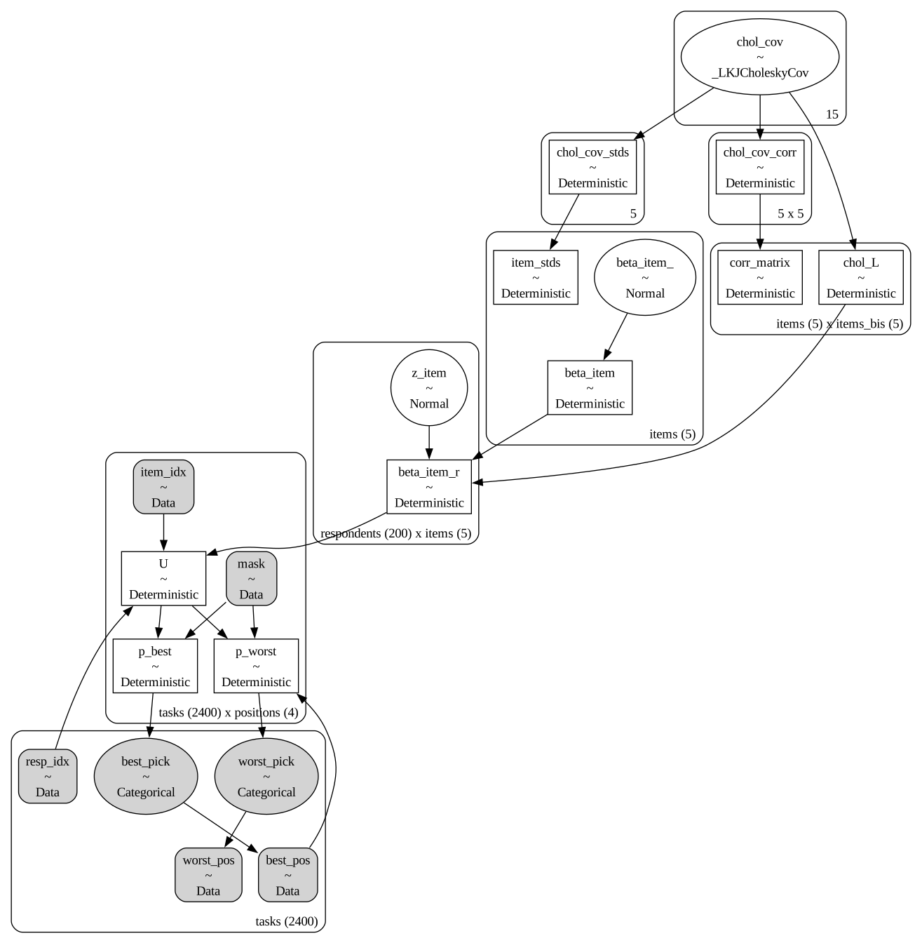
For each task \(t\) a respondent \(r\) sees a subset \(S_t\) of the item pool and picks a best item \(b_t\) and worst item \(w_t\). The Louviere sequential best-worst likelihood decomposes the joint pick as
Item utilities \(U_{rj}\) decompose into a population-level item intercept plus a per-respondent deviation:
with the reference item pinned to \(\beta_{\text{ref}} = 0\) for identification. Only utility contrasts against the reference item are identified — absolute utility levels are arbitrary.
Synthetic data#
generate_maxdiff_data draws subsets uniformly at random (a real field design would use a balanced incomplete block design) and simulates best / worst picks under the Louviere model. It returns a long-format DataFrame and a dictionary of the true utilities we want to recover.
corr = np.array(
    [
        [1.0, 0.7, 0.6, -0.4, -0.3],
        [0.7, 1.0, 0.5, -0.3, -0.3],
        [0.6, 0.5, 1.0, -0.3, -0.2],
        [-0.4, -0.3, -0.3, 1.0, 0.6],
        [-0.3, -0.3, -0.2, 0.6, 1.0],
    ]
)

task_df, ground_truth = generate_maxdiff_data(
    n_respondents=200,
    n_items=5,
    n_tasks_per_resp=12,
    subset_size=4,
    sigma_respondent=0.4,
    random_seed=SEED,
    item_correlation=corr,
)

items = ground_truth["items"]
true_utilities = ground_truth["utilities"]
task_df.head()
| respondent_id | task_id | item_id | is_best | is_worst | |
|---|---|---|---|---|---|
| 0 | r0 | 0 | item_4 | 1 | 0 |
| 1 | r0 | 0 | item_3 | 0 | 0 |
| 2 | r0 | 0 | item_0 | 0 | 1 |
| 3 | r0 | 0 | item_1 | 0 | 0 |
| 4 | r0 | 1 | item_1 | 0 | 0 |
Each row is one shown item in one task. Exactly one row per (respondent_id, task_id) group
carries is_best=1 and one carries is_worst=1.
grouped = task_df.groupby(["respondent_id", "task_id"])
print(f"respondents: {task_df['respondent_id'].nunique()}")
print(f"tasks:       {grouped.ngroups}")
print(f"rows:        {len(task_df)}  (= tasks x subset_size)")
print(f"items:       {len(items)}")
respondents: 200
tasks:       2400
rows:        9600  (= tasks x subset_size)
items:       5
Data format and prepare_maxdiff_data#
The long-format task_df above is the natural export from Sawtooth / Qualtrics / Conjointly. Internally, MaxDiffMixedLogit reshapes it into a padded-plus-mask representation via prepare_maxdiff_data. You can call the helper directly to inspect what the model consumes. This is useful when debugging imports from survey platforms.
from pymc_marketing.customer_choice import prepare_maxdiff_data

arrays = prepare_maxdiff_data(task_df, items=items)

print(f"n_tasks      = {arrays['n_tasks']}")
print(f"n_respondents= {arrays['n_respondents']}")
print(f"n_items      = {arrays['n_items']}")
print(f"k_max        = {arrays['k_max']} (largest subset size)\n")

print("item_idx[:5]   (items shown per task, as ints into `items`):")
print(arrays["item_idx"][:5])
print("\nmask[:5]       (True = real shown item, False = padding):")
print(arrays["mask"][:5])
print("\nbest_pos[:5]   (position 0..k_max-1 of the best pick):")
print(arrays["best_pos"][:5])
print("\nworst_pos[:5]  (position of the worst pick):")
print(arrays["worst_pos"][:5])
print("\nresp_idx[:5]   (respondent index per task):")
print(arrays["resp_idx"][:5])
n_tasks      = 2400
n_respondents= 200
n_items      = 5
k_max        = 4 (largest subset size)

item_idx[:5]   (items shown per task, as ints into `items`):
[[4 3 0 1]
 [1 2 0 4]
 [2 3 0 1]
 [0 4 2 3]
 [3 0 4 1]]

mask[:5]       (True = real shown item, False = padding):
[[ True  True  True  True]
 [ True  True  True  True]
 [ True  True  True  True]
 [ True  True  True  True]
 [ True  True  True  True]]

best_pos[:5]   (position 0..k_max-1 of the best pick):
[0 1 1 3 0]

worst_pos[:5]  (position of the worst pick):
[2 3 3 1 2]

resp_idx[:5]   (respondent index per task):
[0 0 0 0 0]
Ragged subsets and input validation#
Real MaxDiff designs occasionally mix subset sizes within a single study. When a task_df has ragged subsets, prepare_maxdiff_data pads the shorter tasks with the reference item; the mask array records which positions are real so the model ignores padding in the softmax.
The helper also validates the data up front and raises a descriptive ValueError on malformed inputs i.e. missing best/worst picks, duplicate best picks, best == worst in the same task, duplicate items within a task, or items outside the declared pool:
bad_df = task_df.copy()
# Corrupt the first task: remove the best pick
first_task = (bad_df["respondent_id"] == "r0") & (bad_df["task_id"] == 0)
bad_df.loc[first_task, "is_best"] = 0

try:
    prepare_maxdiff_data(bad_df, items=items)
except ValueError as e:
    print(f"Caught expected error:\n  {e}")
Caught expected error:
  Task ('r0', np.int64(0)) has 0 best picks; exactly one is required.
Fit#
model = MaxDiffMixedLogit(task_df=task_df, items=items, full_covariance=True)
idata = model.fit(
    draws=1000,
    tune=1000,
    chains=4,
    target_accept=0.9,
    random_seed=SEED,
)
The rhat statistic is larger than 1.01 for some parameters. This indicates problems during sampling. See https://arxiv.org/abs/1903.08008 for details
The effective sample size per chain is smaller than 100 for some parameters.  A higher number is needed for reliable rhat and ess computation. See https://arxiv.org/abs/1903.08008 for details
pm.model_to_graphviz(model.model)
Parameter recovery#
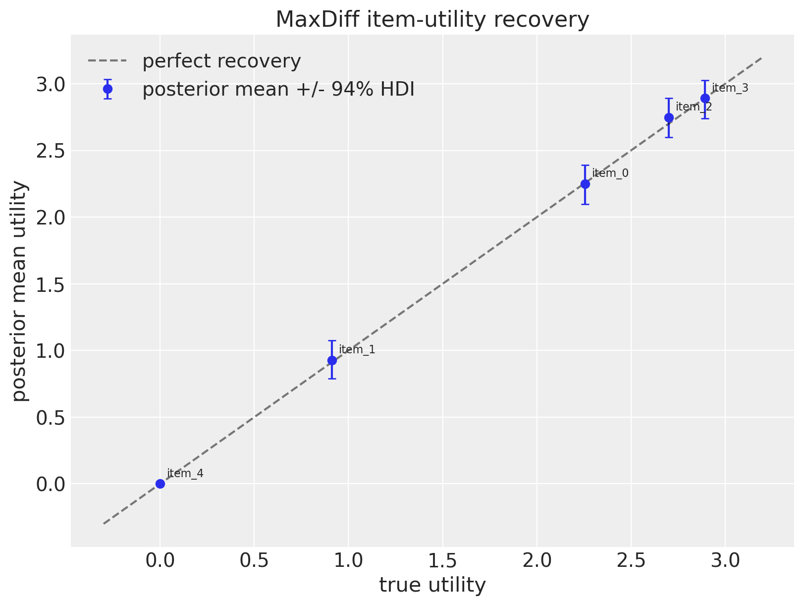
Plot posterior item utilities against the ground truth. The dashed 45° line is perfect recovery.
idata
-
<xarray.Dataset> Size: 989MB Dimensions: (chain: 4, draw: 1000, items: 5, respondents: 200, chol_cov_dim_0: 15, chol_cov_corr_dim_0: 5, chol_cov_corr_dim_1: 5, chol_cov_stds_dim_0: 5, items_bis: 5, tasks: 2400, positions: 4) Coordinates: * chain (chain) int64 32B 0 1 2 3 * draw (draw) int64 8kB 0 1 2 3 4 5 ... 995 996 997 998 999 * items (items) <U6 120B 'item_0' 'item_1' ... 'item_4' * respondents (respondents) <U4 3kB 'r0' 'r1' 'r2' ... 'r198' 'r199' * chol_cov_dim_0 (chol_cov_dim_0) int64 120B 0 1 2 3 4 ... 11 12 13 14 * chol_cov_corr_dim_0 (chol_cov_corr_dim_0) int64 40B 0 1 2 3 4 * chol_cov_corr_dim_1 (chol_cov_corr_dim_1) int64 40B 0 1 2 3 4 * chol_cov_stds_dim_0 (chol_cov_stds_dim_0) int64 40B 0 1 2 3 4 * items_bis (items_bis) <U6 120B 'item_0' 'item_1' ... 'item_4' * tasks (tasks) int64 19kB 0 1 2 3 4 ... 2396 2397 2398 2399 * positions (positions) int64 32B 0 1 2 3 Data variables: (12/13) beta_item_ (chain, draw, items) float64 160kB 2.281 1.022 ... 1.01 z_item (chain, draw, respondents, items) float64 32MB 0.224... chol_cov (chain, draw, chol_cov_dim_0) float64 480kB 0.1498 .... beta_item (chain, draw, items) float64 160kB 2.281 1.022 ... 0.0 chol_cov_corr (chain, draw, chol_cov_corr_dim_0, chol_cov_corr_dim_1) float64 800kB ... chol_cov_stds (chain, draw, chol_cov_stds_dim_0) float64 160kB 0.1... ... ... corr_matrix (chain, draw, items, items_bis) float64 800kB 1.0 ..... item_stds (chain, draw, items) float64 160kB 0.1498 ... 0.3132 beta_item_r (chain, draw, respondents, items) float64 32MB 2.315... U (chain, draw, tasks, positions) float64 307MB 0.2477... p_best (chain, draw, tasks, positions) float64 307MB 0.0325... p_worst (chain, draw, tasks, positions) float64 307MB 0.0 ..... Attributes: created_at: 2026-05-01T20:48:26.954463+00:00 arviz_version: 0.23.0 inference_library: numpyro inference_library_version: 0.19.0 sampling_time: 36.067797 tuning_steps: 1000 pymc_marketing_version: 0.19.3 -
<xarray.Dataset> Size: 154MB Dimensions: (chain: 4, draw: 1000, tasks: 2400) Coordinates: * chain (chain) int64 32B 0 1 2 3 * draw (draw) int64 8kB 0 1 2 3 4 5 6 7 ... 993 994 995 996 997 998 999 * tasks (tasks) int64 19kB 0 1 2 3 4 5 ... 2394 2395 2396 2397 2398 2399 Data variables: best_pick (chain, draw, tasks) float64 77MB -3.424 -0.8513 ... -0.8126 worst_pick (chain, draw, tasks) float64 77MB -1.458 -0.3994 ... -1.279 Attributes: created_at: 2026-05-01T20:48:26.970476+00:00 arviz_version: 0.23.0 -
<xarray.Dataset> Size: 204kB Dimensions: (chain: 4, draw: 1000) Coordinates: * chain (chain) int64 32B 0 1 2 3 * draw (draw) int64 8kB 0 1 2 3 4 5 6 ... 994 995 996 997 998 999 Data variables: acceptance_rate (chain, draw) float64 32kB 0.8874 0.9132 ... 0.9961 0.5653 step_size (chain, draw) float64 32kB 0.09398 0.09398 ... 0.08802 diverging (chain, draw) bool 4kB False False False ... False False energy (chain, draw) float64 32kB 6.1e+03 6.129e+03 ... 6.11e+03 n_steps (chain, draw) int64 32kB 63 63 63 63 63 ... 63 63 63 63 63 tree_depth (chain, draw) int64 32kB 6 6 6 6 6 6 6 6 ... 6 6 6 6 6 6 6 lp (chain, draw) float64 32kB 5.605e+03 ... 5.651e+03 Attributes: created_at: 2026-05-01T20:48:26.969287+00:00 arviz_version: 0.23.0 -
<xarray.Dataset> Size: 58kB Dimensions: (tasks: 2400) Coordinates: * tasks (tasks) int64 19kB 0 1 2 3 4 5 ... 2394 2395 2396 2397 2398 2399 Data variables: best_pick (tasks) int64 19kB 0 1 1 3 0 3 2 3 1 1 1 ... 2 3 2 1 1 3 3 0 2 2 worst_pick (tasks) int64 19kB 2 3 3 1 2 1 1 0 2 2 0 ... 0 1 3 2 2 0 2 2 0 0 Attributes: created_at: 2026-05-01T20:48:26.971090+00:00 arviz_version: 0.23.0 inference_library: numpyro inference_library_version: 0.19.0 sampling_time: 36.067797 tuning_steps: 1000 -
<xarray.Dataset> Size: 96kB Dimensions: (tasks: 2400, positions: 4) Coordinates: * tasks (tasks) int64 19kB 0 1 2 3 4 5 ... 2394 2395 2396 2397 2398 2399 * positions (positions) int64 32B 0 1 2 3 Data variables: item_idx (tasks, positions) int32 38kB 4 3 0 1 1 2 0 4 ... 1 4 0 3 1 3 2 4 mask (tasks, positions) bool 10kB True True True ... True True True best_pos (tasks) int32 10kB 0 1 1 3 0 3 2 3 1 1 1 ... 2 3 2 1 1 3 3 0 2 2 worst_pos (tasks) int32 10kB 2 3 3 1 2 1 1 0 2 2 0 ... 0 1 3 2 2 0 2 2 0 0 resp_idx (tasks) int32 10kB 0 0 0 0 0 0 0 ... 199 199 199 199 199 199 199 Attributes: created_at: 2026-05-01T20:48:26.971905+00:00 arviz_version: 0.23.0 inference_library: numpyro inference_library_version: 0.19.0 sampling_time: 36.067797 tuning_steps: 1000 -
<xarray.Dataset> Size: 461kB
Dimensions:        (row: 9600)
Coordinates:
  * row            (row) int64 77kB 0 1 2 3 4 5 ... 9595 9596 9597 9598 9599
Data variables:
    respondent_id  (row) object 77kB 'r0' 'r0' 'r0' ... 'r199' 'r199' 'r199'
    task_id        (row) int64 77kB 0 0 0 0 1 1 1 1 ... 10 10 10 10 11 11 11 11
    item_id        (row) object 77kB 'item_4' 'item_3' ... 'item_2' 'item_4'
    is_best        (row) int64 77kB 1 0 0 0 0 1 0 0 0 1 ... 0 0 0 0 1 0 0 0 1 0
    is_worst       (row) int64 77kB 0 0 1 0 0 0 0 1 0 0 ... 1 0 1 0 0 0 1 0 0 0
az.summary(idata, var_names=["beta_item", "corr_matrix"], round_to=2)
/Users/nathanielforde/mambaforge/envs/pymc-marketing-dev/lib/python3.12/site-packages/arviz/stats/diagnostics.py:596: RuntimeWarning: invalid value encountered in scalar divide
  (between_chain_variance / within_chain_variance + num_samples - 1) / (num_samples)
/Users/nathanielforde/mambaforge/envs/pymc-marketing-dev/lib/python3.12/site-packages/arviz/stats/diagnostics.py:991: RuntimeWarning: invalid value encountered in scalar divide
  varsd = varvar / evar / 4
| mean | sd | hdi_3% | hdi_97% | mcse_mean | mcse_sd | ess_bulk | ess_tail | r_hat | |
|---|---|---|---|---|---|---|---|---|---|
| beta_item[item_0] | 2.25 | 0.08 | 2.10 | 2.39 | 0.00 | 0.00 | 2438.20 | 2900.25 | 1.00 |
| beta_item[item_1] | 0.93 | 0.08 | 0.79 | 1.07 | 0.00 | 0.00 | 2593.78 | 3280.50 | 1.00 |
| beta_item[item_2] | 2.75 | 0.08 | 2.60 | 2.89 | 0.00 | 0.00 | 2618.02 | 2820.24 | 1.00 |
| beta_item[item_3] | 2.89 | 0.08 | 2.74 | 3.03 | 0.00 | 0.00 | 2987.37 | 2623.99 | 1.00 |
| beta_item[item_4] | 0.00 | 0.00 | 0.00 | 0.00 | 0.00 | NaN | 4000.00 | 4000.00 | NaN |
| corr_matrix[item_0, item_0] | 1.00 | 0.00 | 1.00 | 1.00 | 0.00 | NaN | 4000.00 | 4000.00 | NaN |
| corr_matrix[item_0, item_1] | 0.35 | 0.36 | -0.34 | 0.90 | 0.03 | 0.01 | 143.39 | 484.19 | 1.02 |
| corr_matrix[item_0, item_2] | 0.14 | 0.36 | -0.48 | 0.80 | 0.02 | 0.01 | 369.40 | 843.02 | 1.02 |
| corr_matrix[item_0, item_3] | -0.16 | 0.32 | -0.75 | 0.47 | 0.03 | 0.02 | 110.59 | 75.99 | 1.03 |
| corr_matrix[item_0, item_4] | -0.13 | 0.33 | -0.71 | 0.54 | 0.03 | 0.02 | 123.53 | 94.49 | 1.02 |
| corr_matrix[item_1, item_0] | 0.35 | 0.36 | -0.34 | 0.90 | 0.03 | 0.01 | 143.39 | 484.19 | 1.02 |
| corr_matrix[item_1, item_1] | 1.00 | 0.00 | 1.00 | 1.00 | 0.00 | 0.00 | 3939.55 | 3948.36 | 1.00 |
| corr_matrix[item_1, item_2] | -0.02 | 0.36 | -0.67 | 0.63 | 0.02 | 0.01 | 248.27 | 659.93 | 1.01 |
| corr_matrix[item_1, item_3] | -0.16 | 0.27 | -0.64 | 0.35 | 0.02 | 0.00 | 245.10 | 1251.76 | 1.02 |
| corr_matrix[item_1, item_4] | -0.24 | 0.28 | -0.73 | 0.29 | 0.01 | 0.00 | 423.33 | 1313.43 | 1.01 |
| corr_matrix[item_2, item_0] | 0.14 | 0.36 | -0.48 | 0.80 | 0.02 | 0.01 | 369.40 | 843.02 | 1.02 |
| corr_matrix[item_2, item_1] | -0.02 | 0.36 | -0.67 | 0.63 | 0.02 | 0.01 | 248.27 | 659.93 | 1.01 |
| corr_matrix[item_2, item_2] | 1.00 | 0.00 | 1.00 | 1.00 | 0.00 | 0.00 | 3994.99 | 4000.00 | 1.00 |
| corr_matrix[item_2, item_3] | 0.04 | 0.34 | -0.62 | 0.59 | 0.04 | 0.01 | 66.43 | 313.48 | 1.05 |
| corr_matrix[item_2, item_4] | 0.14 | 0.33 | -0.50 | 0.69 | 0.03 | 0.01 | 114.86 | 565.88 | 1.04 |
| corr_matrix[item_3, item_0] | -0.16 | 0.32 | -0.75 | 0.47 | 0.03 | 0.02 | 110.59 | 75.99 | 1.03 |
| corr_matrix[item_3, item_1] | -0.16 | 0.27 | -0.64 | 0.35 | 0.02 | 0.00 | 245.10 | 1251.76 | 1.02 |
| corr_matrix[item_3, item_2] | 0.04 | 0.34 | -0.62 | 0.59 | 0.04 | 0.01 | 66.43 | 313.48 | 1.05 |
| corr_matrix[item_3, item_3] | 1.00 | 0.00 | 1.00 | 1.00 | 0.00 | 0.00 | 3841.70 | 3868.91 | 1.00 |
| corr_matrix[item_3, item_4] | 0.66 | 0.26 | 0.14 | 0.96 | 0.02 | 0.02 | 163.02 | 395.06 | 1.03 |
| corr_matrix[item_4, item_0] | -0.13 | 0.33 | -0.71 | 0.54 | 0.03 | 0.02 | 123.53 | 94.49 | 1.02 |
| corr_matrix[item_4, item_1] | -0.24 | 0.28 | -0.73 | 0.29 | 0.01 | 0.00 | 423.33 | 1313.43 | 1.01 |
| corr_matrix[item_4, item_2] | 0.14 | 0.33 | -0.50 | 0.69 | 0.03 | 0.01 | 114.86 | 565.88 | 1.04 |
| corr_matrix[item_4, item_3] | 0.66 | 0.26 | 0.14 | 0.96 | 0.02 | 0.02 | 163.02 | 395.06 | 1.03 |
| corr_matrix[item_4, item_4] | 1.00 | 0.00 | 1.00 | 1.00 | 0.00 | 0.00 | 4030.34 | 3399.12 | 1.00 |
Respondent heterogeneity#
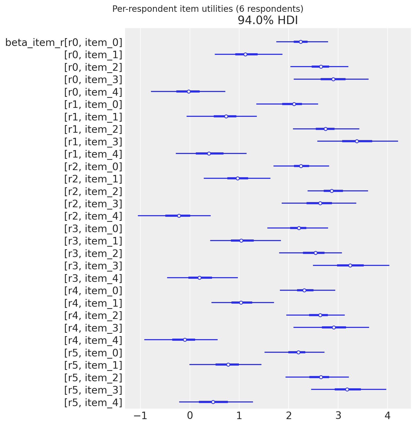
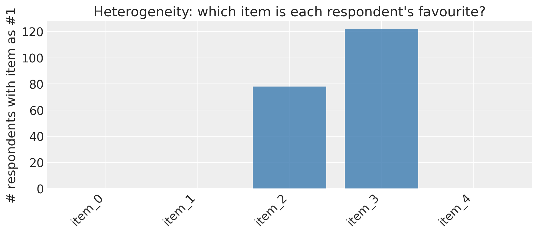
beta_item_r holds per-respondent item utilities. A forest of the first few respondents shows
how strongly preferences vary — the motivation for the hierarchical layer.
Share of preference#
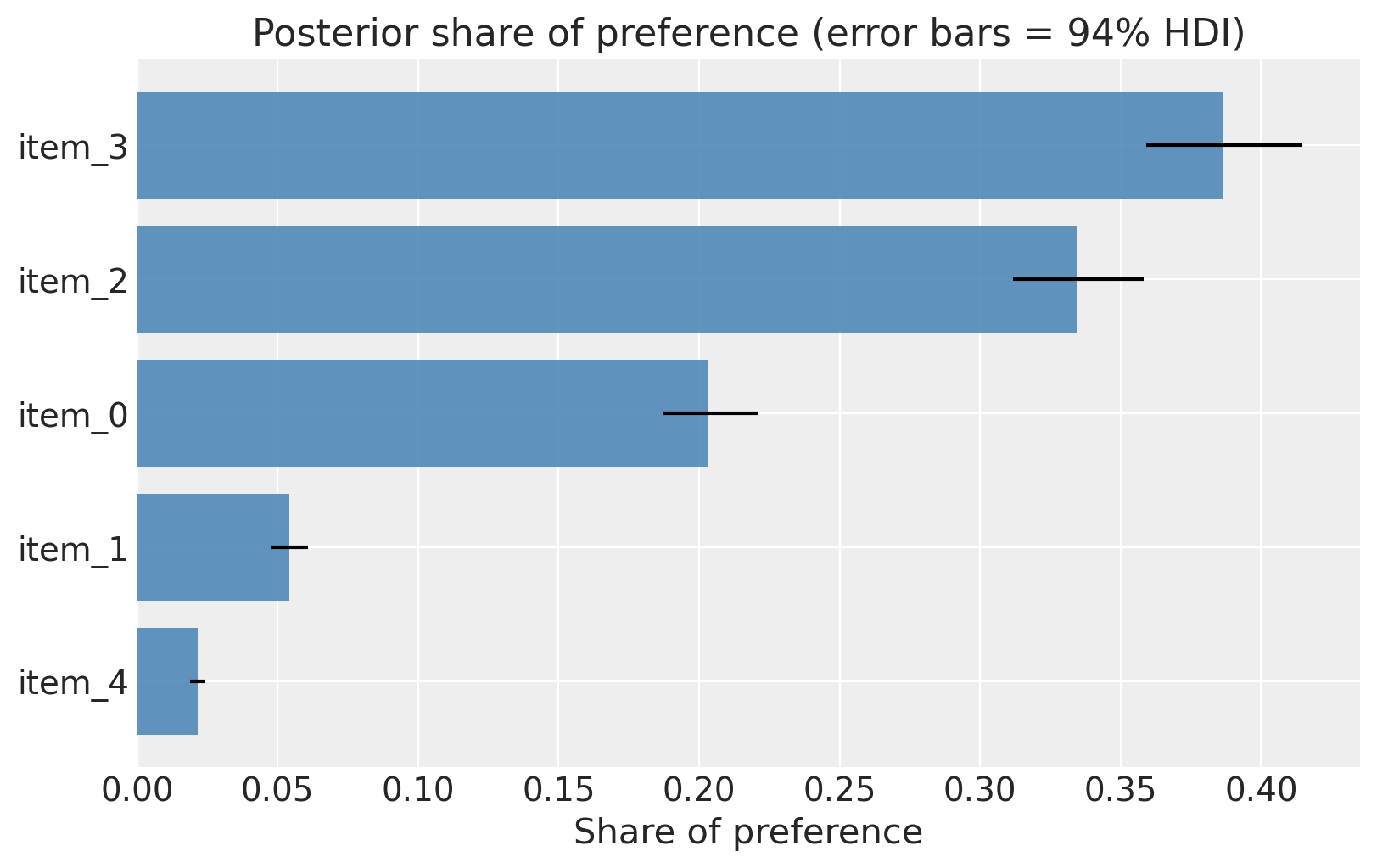
A common consulting deliverable is the share of implied preferences: given the posterior utilities, what fraction of respondents would pick each item if all items were shown together? This is just the softmax of the posterior item utilities averaged over draws.
Counterfactual: restricted-assortment share of preference#
A real business question: if we discontinued items 2, 3 and 4, how would demand shift to the survivors? This is a genuinely out-of-sample prediction — the restricted assortment was never shown during the survey.
apply_intervention answers it by building a synthetic task where every respondent is shown the counterfactual item set, then generatively sampling per-respondent best picks from the posterior. Because beta_item_r captures per-respondent preferences, the resulting substitution pattern is preference-weighted — respondents who liked a dropped item don’t all move to the same survivor.
The bar chart below compares:
Blue (before): the absolute share each surviving item held in the full assortment — i.e. the raw softmax share when all 5 items compete.
Orange (after): the model-predicted share inside the restricted 2-item assortment.
The key insight is IIA (Independence of Irrelevant Alternatives): under a pure softmax the ratio between item_0 and item_1 is unchanged by removing competitors, but the absolute level of each item’s share rises substantially once the three dropped items no longer absorb probability mass.
import pandas as pd

# Counterfactual assortment: items 3, 2 and 4 are discontinued.
dropped = {"item_3", "item_2", "item_4"}
restricted_items = [it for it in items if it not in dropped]
print(f"Restricted assortment ({len(restricted_items)} items): {restricted_items}")

# Build a counterfactual task_df: every respondent sees the restricted set in one task.
# No is_best / is_worst columns needed -- apply_intervention auto-generates dummy flags.
cf_rows = []
for r in task_df["respondent_id"].unique():
    for it in restricted_items:
        cf_rows.append({"respondent_id": r, "task_id": 0, "item_id": it})
cf_df = pd.DataFrame(cf_rows)

# apply_intervention wraps predict_choices and stores the result as model.intervention_idata.
cf_preds = model.apply_intervention(cf_df, random_seed=SEED)

# best_pick shape: (chain, draw, tasks). Here tasks == n_respondents.
best_positions = cf_preds["best_pick"].values
restricted_arr = np.array(restricted_items)
best_item_per_draw = restricted_arr[best_positions]  # (chain, draw, respondents)

# Model-based share: fraction of (chain, draw, respondent) picks per item.
cf_share_per_draw = np.stack(
    [(best_item_per_draw == it).mean(axis=-1) for it in restricted_items]
)  # (items, chain, draw)
cf_share_mean = cf_share_per_draw.mean(axis=(1, 2))
cf_share_hdi = np.quantile(
    cf_share_per_draw.reshape(len(restricted_items), -1), [0.03, 0.97], axis=1
)

# Full-pool baseline: absolute (non-renormalised) share of each surviving item
# in the original full-assortment softmax.  We deliberately do NOT renormalise
# here -- that would reproduce the IIA ratio and make the comparison circular.
full_share_map = dict(zip(items, share_mean, strict=True))
full_share_restricted = np.array([full_share_map[it] for it in restricted_items])

fig, ax = plt.subplots(figsize=(7, 4))
x = np.arange(len(restricted_items))
w = 0.35
ax.bar(
    x - w / 2,
    full_share_restricted,
    w,
    label="Full assortment (before)",
    color="steelblue",
    alpha=0.85,
)
ax.bar(
    x + w / 2,
    cf_share_mean,
    w,
    label="Restricted assortment (after)",
    color="darkorange",
    alpha=0.85,
)
ax.errorbar(
    x + w / 2,
    cf_share_mean,
    yerr=np.abs(cf_share_hdi - cf_share_mean),
    fmt="none",
    color="black",
    capsize=3,
    linewidth=1,
)
ax.set_xticks(x)
ax.set_xticklabels(restricted_items)
ax.set_ylabel("Share of preference")
ax.set_title(
    "Absolute share before and after dropping {" + ", ".join(sorted(dropped)) + "}"
)
ax.legend()
ax.set_ylim(0, 1)
fig.tight_layout()
plt.show()

print("\nFull-pool absolute share (surviving items):")
for it, s in zip(restricted_items, full_share_restricted, strict=True):
    print(f"  {it}: {s:.3f}")
print("\nRestricted-assortment share (model-based):")
for it, s in zip(restricted_items, cf_share_mean, strict=True):
    print(f"  {it}: {s:.3f}")
print(
    "\nNote: the ratio between surviving items is preserved (IIA property), "
    "but absolute shares rise substantially when competitors are removed."
)
Restricted assortment (2 items): ['item_0', 'item_1']
/var/folders/__/ng_3_9pn1f11ftyml_qr69vh0000gn/T/ipykernel_36804/2012962254.py:17: UserWarning: Neither 'is_best' nor 'is_worst' found in task_df. Dummy flags have been auto-generated (the assignment is arbitrary and depends on the current row order within each task group). These flags are not used during prediction but satisfy the data validator. Provide explicit flag columns if true best/worst labels are needed.
  cf_preds = model.apply_intervention(cf_df, random_seed=SEED)
/var/folders/__/ng_3_9pn1f11ftyml_qr69vh0000gn/T/ipykernel_36804/2012962254.py:75: UserWarning: The figure layout has changed to tight
  fig.tight_layout()
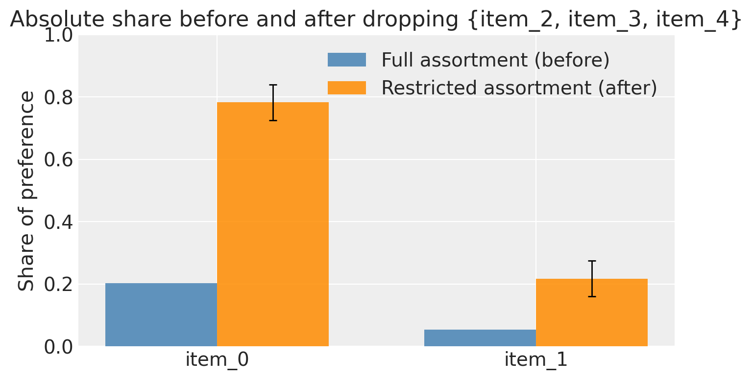
Full-pool absolute share (surviving items):
  item_0: 0.203
  item_1: 0.054

Restricted-assortment share (model-based):
  item_0: 0.783
  item_1: 0.217

Note: the ratio between surviving items is preserved (IIA property), but absolute shares rise substantially when competitors are removed.
beta_r_mean = (
    idata["posterior"]["beta_item_r"].mean(dim=("chain", "draw")).values
)  # (R, I)
top_item_idx = np.argmax(beta_r_mean, axis=1)
top_item_counts = (
    pd.Series([items[i] for i in top_item_idx], name="top_item")
    .value_counts()
    .reindex(items, fill_value=0)
)

fig, ax = plt.subplots(figsize=(9, 4))
ax.bar(range(len(items)), top_item_counts.values, color="steelblue", alpha=0.85)
ax.set_xticks(range(len(items)))
ax.set_xticklabels(top_item_counts.index, rotation=45, ha="right")
ax.set_ylabel("# respondents with item as #1")
ax.set_title("Heterogeneity: which item is each respondent's favourite?")
plt.tight_layout()
plt.show()
/var/folders/__/ng_3_9pn1f11ftyml_qr69vh0000gn/T/ipykernel_36804/2766163016.py:17: UserWarning: The figure layout has changed to tight
  plt.tight_layout()
Caveats and follow-ups#
Design: real MaxDiff studies use balanced incomplete block designs (Sawtooth/Lighthouse). This model does not care which design produced the data — but efficiency is much higher under balanced rotations.
Item-attribute part-worths: when items share structure (price, brand, feature levels), a linear utility over item covariates \(U_j = x_j^\top \beta\) gains efficiency — see Part II below.
sample_posterior_predictive vs predict_choices / apply_intervention#
The Louviere model is sequential: the worst pick is drawn from the remaining items after the best has been removed. In the PyMC graph this is achieved by masking the chosen best position out of the worst-pick softmax, using best_pos as a pm.Data node.
sample_posterior_predictive therefore produces a partially conditioned joint:
best_pickis sampled correctly from \(\operatorname{softmax}(U)\).worst_pickis conditioned on the observedbest_pos(the value in the training data), not on the freshly sampledbest_pick.
This means the two draws can designate the same position i.e. the joint is incoherent for generative use. Instead for generative usage predict_choices and apply_intervention sample best first, then condition worst on the sampled best, so the joint is always coherent. All counterfactual work in this notebook uses apply_intervention for exactly this reason. The table below summarises when each method is appropriate:
Task |
Correct method |
|---|---|
In-sample PPC — does the model reproduce training worst picks given observed bests? |
|
Counterfactual / out-of-sample — coherent joint \((b, w)\) draws |
|
Part II — MaxDiff with attribute part-worths#
So far each item carried its own free utility. In conjoint-style MaxDiff we instead decompose utility into attribute part-worths:
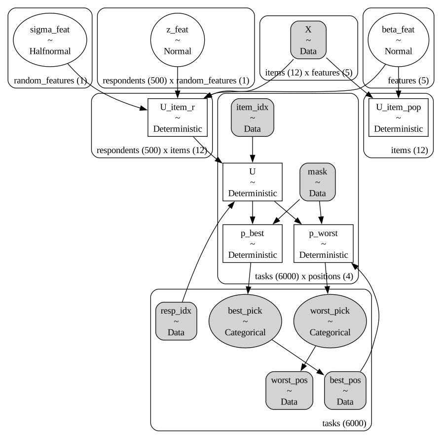
where \(X_i\) is a row of attribute features (brand dummies, price, quality score, …) and \(\beta_{\text{feat}}\) is a vector of population-level part-worths. This buys three things the item-intercept model cannot give:
Extrapolation to new items. A hypothetical SKU outside the training pool gets a utility from its attributes alone — no need to re-survey.
Attribute-level inference. The posterior on \(\beta_{\text{feat}}\) tells us what drives preference, not just which item is preferred.
Heterogeneity on a chosen subspace. Pass
random_attributes=[...]to let respondents vary on a strict subset of features (e.g. price sensitivity) while sharing population beliefs on the rest.
Identification comes from ~ 0 + ... in the patsy formula (drop the global intercept) plus a sum-to-zero constraint on the implied per-item utilities. No reference item is needed.
from pymc_marketing.customer_choice import generate_maxdiff_conjoint_data

task_df_pw, attrs, gt = generate_maxdiff_conjoint_data(
    n_respondents=500,
    n_items=12,
    n_tasks_per_resp=12,
    subset_size=4,
    sigma_respondent=0.4,
    random_attributes=["price"],
    random_seed=SEED,
)

print("Items + attributes:")
print(attrs)
print("\nFeature names (after patsy expansion):", gt["feature_names"])
print("Ground-truth betas:", dict(zip(gt["feature_names"], gt["betas"], strict=True)))
Items + attributes:
        brand     price   quality
item_id
item_0      A  0.761140  0.878450
item_1      C  0.786064 -0.049926
item_2      B  0.128114 -0.184862
item_3      B  0.450386 -0.680930
item_4      B  0.370798  1.222541
item_5      C  0.926765 -0.154529
item_6      A  0.643865 -0.428328
item_7      C  0.822762 -0.352134
item_8      A  0.443414  0.532309
item_9      A  0.227239  0.365444
item_10     B  0.554585  0.412733
item_11     C  0.063817  0.430821

Feature names (after patsy expansion): ['C(brand)[A]', 'C(brand)[B]', 'C(brand)[C]', 'price', 'quality']
Ground-truth betas: {'C(brand)[A]': np.float64(2.1416476008704612), 'C(brand)[B]': np.float64(-0.4064150163846156), 'C(brand)[C]': np.float64(-0.5122427290715373), 'price': np.float64(-0.8137727282478777), 'quality': np.float64(0.6159794225754956)}
model_pw = MaxDiffMixedLogit(
    task_df=task_df_pw,
    items=gt["items"],
    item_attributes=attrs,
    utility_formula="~ 0 + C(brand) + price + quality",
    random_attributes=["price"],
)

idata_pw = model_pw.fit(
    draws=1000,
    tune=1000,
    chains=4,
    target_accept=0.9,
    random_seed=SEED,
)
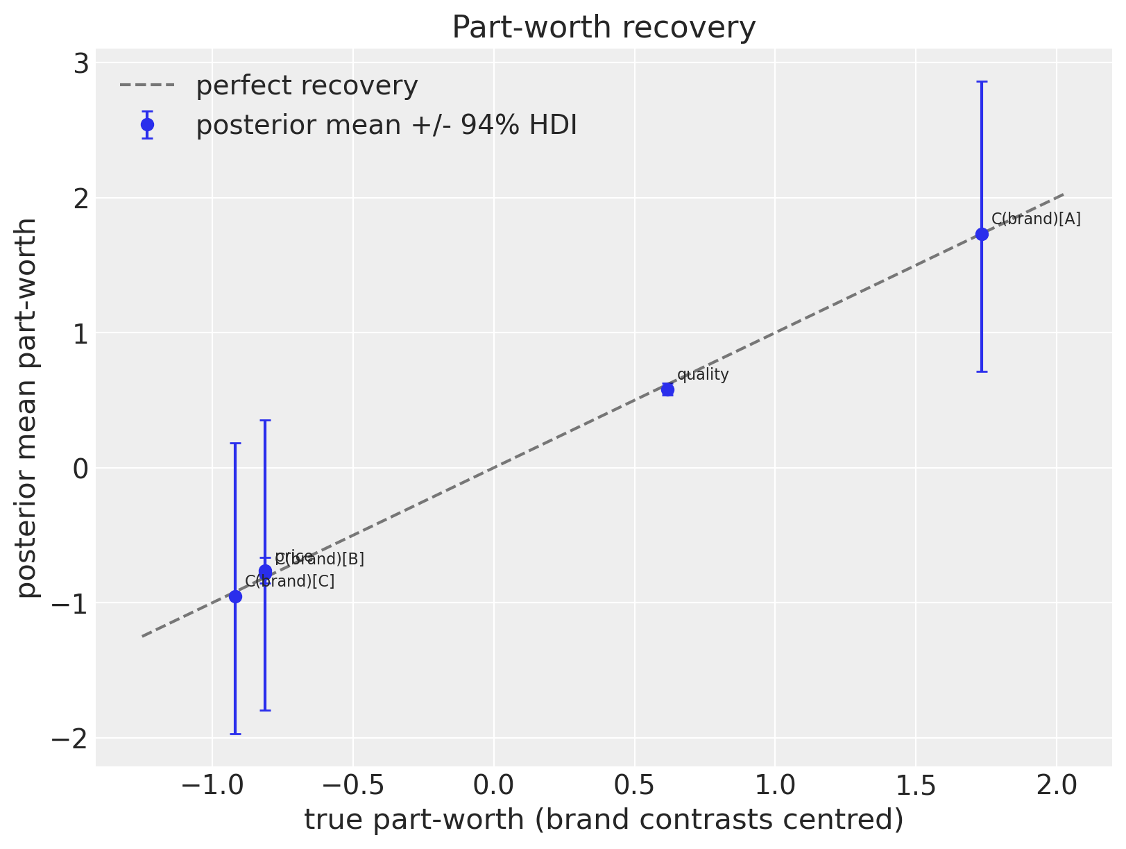
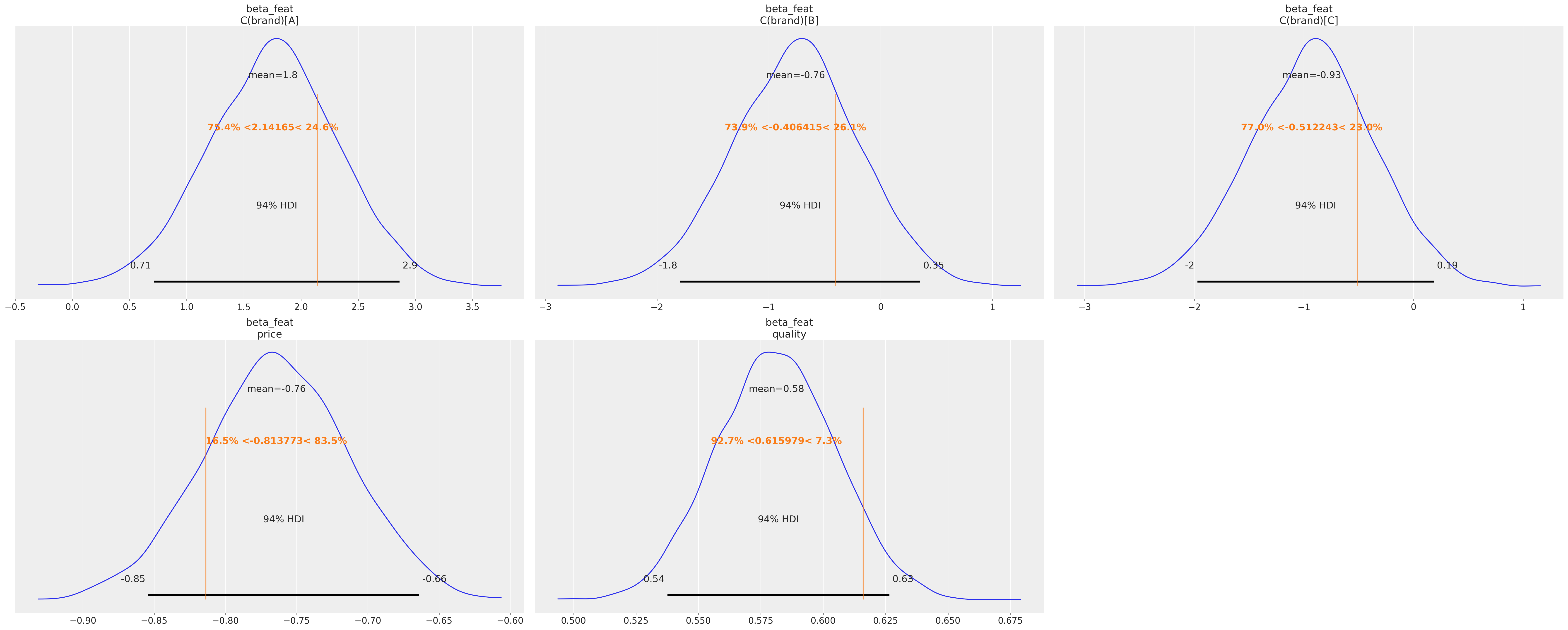
Recovery — population part-worths#
Compare the posterior mean of beta_feat against the simulated ground truth. Brand dummies share an unidentified global location (only contrasts are identified via ~ 0 + ...), so we compare centred values; price and quality recover on absolute scale.
feature_names = model_pw.feature_names
beta_post = idata_pw["posterior"]["beta_feat"]  # (chain, draw, features)
beta_mean = beta_post.mean(dim=("chain", "draw")).values
beta_hdi = az.hdi(beta_post, hdi_prob=0.94)["beta_feat"].values  # (features, 2)
truth = np.asarray(gt["betas"])

# Centre brand dummies (location is unidentified within the brand group).
is_brand = np.array([f.startswith("C(brand)") for f in feature_names])
truth_plot = truth.copy()
mean_plot = beta_mean.copy()
hdi_plot = beta_hdi.copy()
truth_plot[is_brand] -= truth_plot[is_brand].mean()
mean_plot[is_brand] -= mean_plot[is_brand].mean()
hdi_plot[is_brand] -= mean_plot[is_brand].mean()  # shift HDI by same amount

fig, ax = plt.subplots(figsize=(8, 6))
yerr = np.abs(hdi_plot.T - mean_plot)
ax.errorbar(
    truth_plot,
    mean_plot,
    yerr=yerr,
    fmt="o",
    capsize=3,
    label="posterior mean +/- 94% HDI",
)
lo = min(truth_plot.min(), mean_plot.min()) - 0.3
hi = max(truth_plot.max(), mean_plot.max()) + 0.3
ax.plot([lo, hi], [lo, hi], "k--", alpha=0.5, label="perfect recovery")
for i, name in enumerate(feature_names):
    ax.annotate(
        name,
        (truth_plot[i], mean_plot[i]),
        fontsize=8,
        xytext=(5, 5),
        textcoords="offset points",
    )
ax.set_xlabel("true part-worth (brand contrasts centred)")
ax.set_ylabel("posterior mean part-worth")
ax.set_title("Part-worth recovery")
ax.legend()
plt.show()
az.summary(
    idata_pw,
    var_names=["beta_feat", "U_item_pop", "sigma_feat"],
    round_to=2,
)
| mean | sd | hdi_3% | hdi_97% | mcse_mean | mcse_sd | ess_bulk | ess_tail | r_hat | |
|---|---|---|---|---|---|---|---|---|---|
| beta_feat[C(brand)[A]] | 1.75 | 0.57 | 0.71 | 2.86 | 0.01 | 0.01 | 2109.24 | 2407.61 | 1.00 |
| beta_feat[C(brand)[B]] | -0.76 | 0.57 | -1.79 | 0.35 | 0.01 | 0.01 | 2092.10 | 2508.61 | 1.00 |
| beta_feat[C(brand)[C]] | -0.93 | 0.57 | -1.97 | 0.19 | 0.01 | 0.01 | 2105.75 | 2489.38 | 1.00 |
| beta_feat[price] | -0.76 | 0.05 | -0.85 | -0.66 | 0.00 | 0.00 | 6777.19 | 2954.06 | 1.00 |
| beta_feat[quality] | 0.58 | 0.02 | 0.54 | 0.63 | 0.00 | 0.00 | 9291.99 | 3071.91 | 1.00 |
| U_item_pop[item_0] | 1.96 | 0.03 | 1.90 | 2.03 | 0.00 | 0.00 | 5227.57 | 3529.12 | 1.00 |
| U_item_pop[item_1] | -1.28 | 0.02 | -1.33 | -1.24 | 0.00 | 0.00 | 4832.31 | 3239.45 | 1.00 |
| U_item_pop[item_2] | -0.69 | 0.03 | -0.74 | -0.64 | 0.00 | 0.00 | 5044.42 | 3715.66 | 1.00 |
| U_item_pop[item_3] | -1.23 | 0.03 | -1.28 | -1.17 | 0.00 | 0.00 | 5667.21 | 3360.18 | 1.00 |
| U_item_pop[item_4] | -0.06 | 0.03 | -0.12 | -0.00 | 0.00 | 0.00 | 5921.93 | 3483.34 | 1.00 |
| U_item_pop[item_5] | -1.45 | 0.03 | -1.50 | -1.40 | 0.00 | 0.00 | 5078.43 | 3208.73 | 1.00 |
| U_item_pop[item_6] | 1.29 | 0.03 | 1.23 | 1.35 | 0.00 | 0.00 | 4816.45 | 3048.63 | 1.00 |
| U_item_pop[item_7] | -1.49 | 0.03 | -1.54 | -1.44 | 0.00 | 0.00 | 5294.32 | 3206.45 | 1.00 |
| U_item_pop[item_8] | 2.00 | 0.03 | 1.95 | 2.05 | 0.00 | 0.00 | 4709.77 | 2541.81 | 1.00 |
| U_item_pop[item_9] | 2.07 | 0.03 | 2.01 | 2.13 | 0.00 | 0.00 | 4913.63 | 2711.21 | 1.00 |
| U_item_pop[item_10] | -0.67 | 0.02 | -0.71 | -0.63 | 0.00 | 0.00 | 4306.31 | 3230.06 | 1.00 |
| U_item_pop[item_11] | -0.45 | 0.03 | -0.52 | -0.39 | 0.00 | 0.00 | 6026.69 | 3469.42 | 1.00 |
| sigma_feat[price] | 0.23 | 0.12 | 0.00 | 0.41 | 0.01 | 0.00 | 437.80 | 748.23 | 1.01 |
az.plot_posterior(
    idata_pw,
    var_names=["beta_feat"],
    ref_val=list(gt["betas"]),
);
Attribute importance#
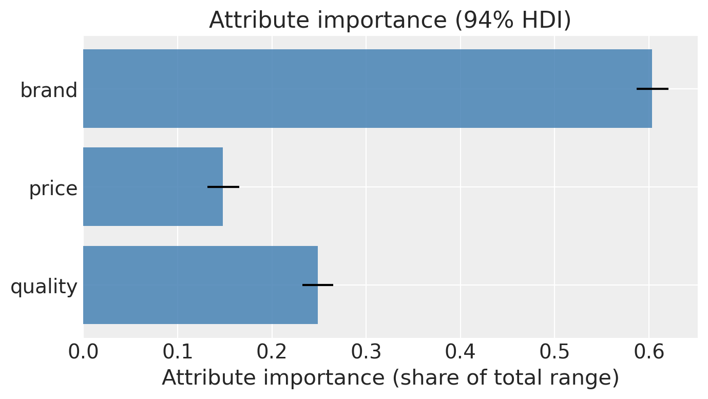
A standard conjoint deliverable. Within each attribute, take the range of part-worths (max − min across its levels for categoricals, or the part-worth times the observed range for continuous attributes), then normalise so the importances sum to 1.
# Posterior draws of beta_feat, shape (samples, features)
beta_draws_pw = (
    idata_pw["posterior"]["beta_feat"]
    .stack(sample=("chain", "draw"))
    .transpose("sample", "features")
    .values
)

attr_groups = {
    "brand": [i for i, f in enumerate(feature_names) if f.startswith("C(brand)")],
    "price": [feature_names.index("price")],
    "quality": [feature_names.index("quality")],
}
# Continuous attributes: importance = |beta| * (observed range across items)
ranges = {
    "price": float(attrs["price"].max() - attrs["price"].min()),
    "quality": float(attrs["quality"].max() - attrs["quality"].min()),
}

importance_draws = {}
for name, idxs in attr_groups.items():
    if name == "brand":
        # Range of brand part-worths per draw
        importance_draws[name] = beta_draws_pw[:, idxs].max(axis=1) - beta_draws_pw[
            :, idxs
        ].min(axis=1)
    else:
        importance_draws[name] = np.abs(beta_draws_pw[:, idxs[0]]) * ranges[name]

stack = np.stack([importance_draws[k] for k in attr_groups])  # (3, samples)
shares = stack / stack.sum(axis=0, keepdims=True)  # normalise per draw
share_mean_pw = shares.mean(axis=1)
share_hdi_pw = np.quantile(shares, [0.03, 0.97], axis=1)

fig, ax = plt.subplots(figsize=(7, 4))
ax.barh(
    list(attr_groups),
    share_mean_pw,
    xerr=np.abs(share_hdi_pw - share_mean_pw),
    color="steelblue",
    alpha=0.85,
)
ax.set_xlabel("Attribute importance (share of total range)")
ax.set_title("Attribute importance (94% HDI)")
ax.invert_yaxis()
plt.tight_layout()
plt.show()
/var/folders/__/ng_3_9pn1f11ftyml_qr69vh0000gn/T/ipykernel_36804/3410986749.py:46: UserWarning: The figure layout has changed to tight
  plt.tight_layout()
Extrapolation to a brand-new item#
A unique selling point of part-worths: we can score a hypothetical SKU that was never shown in the survey. We just need its attribute row. Apply the same patsy formula to the new row and use the posterior of beta_feat to get a full posterior over the new item’s utility. This can, in turn, be plugged directly into a share-of-preference calculation against the existing items.
# Score a brand-new item: brand "B", aggressive price 0.10, average quality 0.0.
new_item = pd.DataFrame(
    [{"brand": "B", "price": 0.10, "quality": 0.0}],
    index=pd.Index(["item_NEW"], name="item_id"),
)

# score_new_items encodes the new row via the fitted patsy formula, computes posterior
# utilities from beta_feat, and returns share-of-preference over the extended pool.
scored = model_pw.score_new_items(new_item)

# scored.coords["items"] = training items + ["item_NEW"]
all_items = list(scored.coords["items"].values)
share_mean_new = scored["share_of_preference"].mean(dim=("chain", "draw")).values

order_new = np.argsort(share_mean_new)[::-1]
fig, ax = plt.subplots(figsize=(8, 5))
y_pos = np.arange(len(all_items))
colors = [
    "darkorange" if all_items[i] == "item_NEW" else "steelblue" for i in order_new
]
ax.barh(
    y_pos,
    share_mean_new[order_new],
    color=colors,
    alpha=0.85,
)
ax.set_yticks(y_pos)
ax.set_yticklabels([all_items[i] for i in order_new])
ax.invert_yaxis()
ax.set_xlabel("Share of preference")
ax.set_title("Share of preference incl. brand-new SKU 'item_NEW' (orange)")
plt.tight_layout()
plt.show()

new_idx = all_items.index("item_NEW")
print(f"New item posterior share: mean={share_mean_new[new_idx]:.3f}")
/var/folders/__/ng_3_9pn1f11ftyml_qr69vh0000gn/T/ipykernel_36804/4087995360.py:32: UserWarning: The figure layout has changed to tight
  plt.tight_layout()
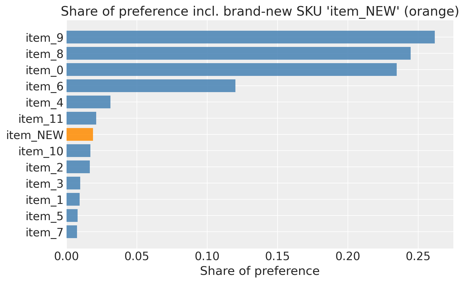
New item posterior share: mean=0.019
pm.model_to_graphviz(model_pw.model)
%load_ext watermark
%watermark -n -u -v -iv -w -p pymc_marketing
Last updated: Fri May 01 2026

Python implementation: CPython
Python version       : 3.12.12
IPython version      : 9.8.0

pymc_marketing: 0.19.3

pandas        : 2.3.3
arviz         : 0.23.0
pymc          : 5.28.2
numpy         : 2.3.5
matplotlib    : 3.10.8
pymc_marketing: 0.19.3

Watermark: 2.5.0