Shifted Beta Geometric model with individual customer data

In this notebook we replicate the main results and figures from

Fader, P. S., & Hardie, B. G. (2007). How to project customer retention. Journal of Interactive Marketing, 21(1), 76-90. https://journals.sagepub.com/doi/pdf/10.1002/dir.20074

The authors describe the Shifted Beta Geometric (sBG) model for customer behavior in a discrete contractual setting. It assumes that:

• At the end of each period, a customer has a probability theta of renewing the contract and 1-theta of cancelling

• The probability theta does not change over time for a given customer

• The probability theta varies across customers according to a Beta prior distribution with hyperparameters alpha and beta.

import arviz as az
import matplotlib.pyplot as plt
import numpy as np
import pandas as pd
import xarray as xr

from pymc_marketing import clv

az.style.use("arviz-darkgrid")

Recreating the dataset

The dataset contains the percentage of customers still enrolled in the service after each time period. There are two distinct groups of users: regular and high-end, believed to have different attrition rates. Each group had 1000 customers at the start.

As in the original paper, we will fit the data from the first 7 time periods only, and use the following periods for validation.

df = pd.DataFrame({
    "regular": [100.0, 63.1, 46.8, 38.2, 32.6, 28.9, 26.2, 24.1, 22.3, 20.7, 19.4, 18.3, 17.3],
    "highend": [100.0, 86.9, 74.3, 65.3, 59.3, 55.1, 51.7, 49.1, 46.8, 44.5, 42.7, 40.9, 39.4],
})
df

	regular	highend
0	100.0	100.0
1	63.1	86.9
2	46.8	74.3
3	38.2	65.3
4	32.6	59.3
5	28.9	55.1
6	26.2	51.7
7	24.1	49.1
8	22.3	46.8
9	20.7	44.5
10	19.4	42.7
11	18.3	40.9
12	17.3	39.4

The implemented pymc-marketing model fits each individual theta, in contrast to the paper approach where the inidividual parameters are marginalized out.

For our analysis we wil have to create a synthetic dataset with individual data, following the aggregate group trends.

def individual_data_from_percentage_alive(percentage_alive, initial_customers):
    n_alive = np.asarray(percentage_alive / 100 * initial_customers, dtype=int)

    died_at = np.zeros((initial_customers,), dtype=int)
    counter = 0
    for t, diff in enumerate((n_alive[:-1] - n_alive[1:]), start=1):
        died_at[counter:counter+diff] = t
        counter += diff

    censoring_t = t+1
    died_at[counter:] = censoring_t

    return died_at

T = 8  # In the paper only the first 7 years are included in the model

truncated_df = df[:T]
initial_customers = 1000  # Seems to be what F&H use, according to Appendix B
churn_highend = individual_data_from_percentage_alive(truncated_df["highend"], initial_customers)
churn_regular = individual_data_from_percentage_alive(truncated_df["regular"], initial_customers)
churn_regular[::10]

array([1, 1, 1, 1, 1, 1, 1, 1, 1, 1, 1, 1, 1, 1, 1, 1, 1, 1, 1, 1, 1, 1,
       1, 1, 1, 1, 1, 1, 1, 1, 1, 1, 1, 1, 1, 1, 1, 2, 2, 2, 2, 2, 2, 2,
       2, 2, 2, 2, 2, 2, 2, 2, 2, 2, 3, 3, 3, 3, 3, 3, 3, 3, 4, 4, 4, 4,
       4, 4, 5, 5, 5, 5, 6, 6, 7, 7, 8, 8, 8, 8, 8, 8, 8, 8, 8, 8, 8, 8,
       8, 8, 8, 8, 8, 8, 8, 8, 8, 8, 8, 8])

Customers which haven’t churned have t_churn == T == 8. The model will handle these differently, as their lifetimes are censored.

Fitting the sBG models for high end and regular users

dataset_highend = pd.DataFrame({
    'customer_id': np.arange(initial_customers),
    't_churn': churn_highend,
    'T': T,
})

highend_users = clv.ShiftedBetaGeoModelIndividual(
    data = dataset_highend
)
highend_users.build_model()
highend_users

Shifted-Beta-Geometric Model (Individual Customers)
         alpha ~ HalfFlat()
          beta ~ HalfFlat()
         theta ~ Beta(alpha, beta)
churn_censored ~ Censored(Geometric(theta), -inf, <constant>)

dataset_regular = pd.DataFrame({
    'customer_id': np.arange(initial_customers),
    't_churn': churn_regular,
    'T': T,
})

regular_users = clv.ShiftedBetaGeoModelIndividual(
    data = dataset_regular
)
regular_users.build_model()
regular_users

Shifted-Beta-Geometric Model (Individual Customers)
         alpha ~ HalfFlat()
          beta ~ HalfFlat()
         theta ~ Beta(alpha, beta)
churn_censored ~ Censored(Geometric(theta), -inf, <constant>)

highend_users.fit()
regular_users.fit();

Auto-assigning NUTS sampler...
Initializing NUTS using jitter+adapt_diag...
Multiprocess sampling (4 chains in 4 jobs)
NUTS: [alpha, beta, theta]

100.00% [8000/8000 00:21<00:00 Sampling 4 chains, 0 divergences]

Sampling 4 chains for 1_000 tune and 1_000 draw iterations (4_000 + 4_000 draws total) took 21 seconds.
The rhat statistic is larger than 1.01 for some parameters. This indicates problems during sampling. See https://arxiv.org/abs/1903.08008 for details
The effective sample size per chain is smaller than 100 for some parameters.  A higher number is needed for reliable rhat and ess computation. See https://arxiv.org/abs/1903.08008 for details
Sampling: [churn_censored]

100.00% [4000/4000 00:00<00:00]

Auto-assigning NUTS sampler...
Initializing NUTS using jitter+adapt_diag...
Multiprocess sampling (4 chains in 4 jobs)
NUTS: [alpha, beta, theta]

100.00% [8000/8000 00:14<00:00 Sampling 4 chains, 0 divergences]

Sampling 4 chains for 1_000 tune and 1_000 draw iterations (4_000 + 4_000 draws total) took 14 seconds.
The rhat statistic is larger than 1.01 for some parameters. This indicates problems during sampling. See https://arxiv.org/abs/1903.08008 for details
The effective sample size per chain is smaller than 100 for some parameters.  A higher number is needed for reliable rhat and ess computation. See https://arxiv.org/abs/1903.08008 for details
Sampling: [churn_censored]

100.00% [4000/4000 00:00<00:00]

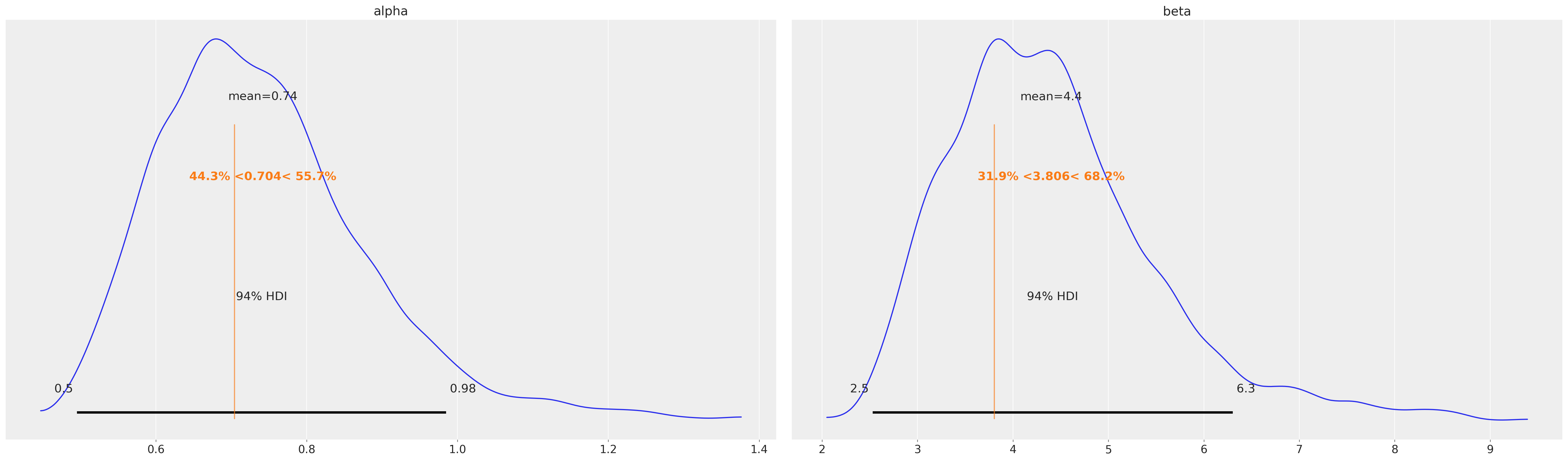
Contrasting posterior inferences with the repo MLE estimates

The sBG model has 2 population parameters of interest: alpha and beta. These parameters define the population distribution of the individual customer’s churn rates theta. The larger the values of alpha and beta the more homogenous the churn rates are across different customers.

The ratio of alpha to beta tells us the expected churn rates. If alpha/beta == 0.1, we expect the average customer to have a 0.1 probability of churning between each time period.

# MLE estimates from the paper
ref_val = {
    "highend": [0.704, 3.806],
    "regular": [0.688, 1.182],
}

highend_users.fit_summary(var_names=["alpha", "beta"])

	mean	sd	hdi_3%	hdi_97%	mcse_mean	mcse_sd	ess_bulk	ess_tail	r_hat
alpha	0.740	0.131	0.529	0.990	0.012	0.009	122.0	166.0	1.02
beta	4.369	1.004	2.765	6.236	0.091	0.066	129.0	191.0	1.02

az.plot_posterior(
    highend_users.fit_result,
    var_names=["alpha", "beta"],
    ref_val=ref_val["highend"]
);

regular_users.fit_summary(var_names=["alpha", "beta"])

	mean	sd	hdi_3%	hdi_97%	mcse_mean	mcse_sd	ess_bulk	ess_tail	r_hat
alpha	0.729	0.071	0.605	0.868	0.005	0.004	171.0	555.0	1.03
beta	1.244	0.167	0.937	1.550	0.013	0.009	157.0	478.0	1.03

az.plot_posterior(
    regular_users.fit_result,
    var_names=["alpha", "beta"],
    ref_val=ref_val["regular"]
);

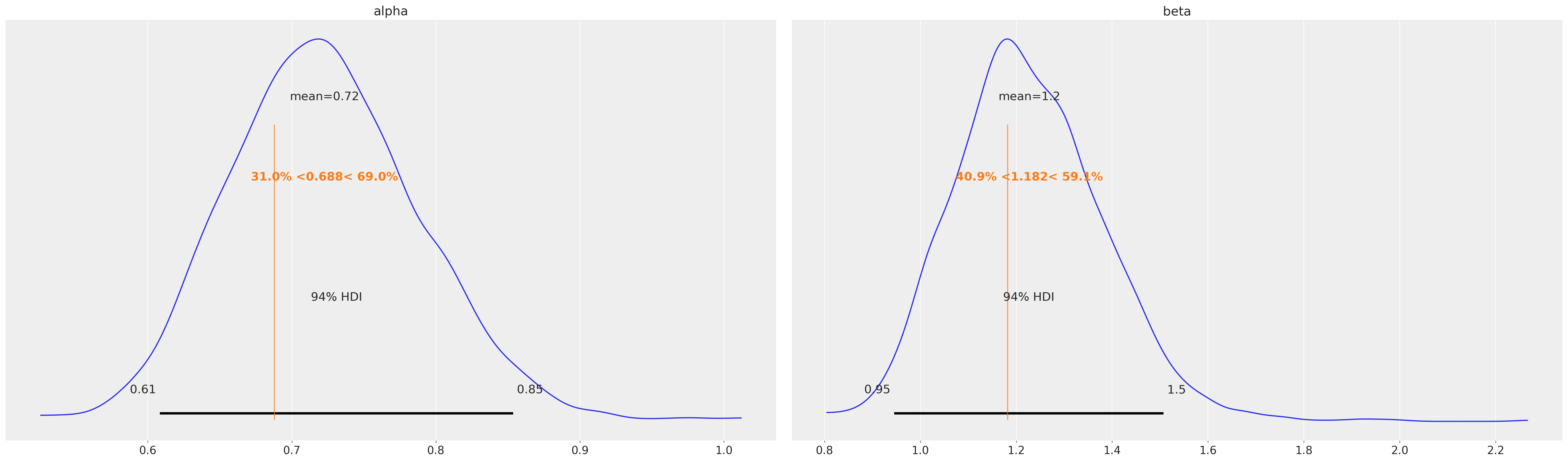
The model fitting agrees with the Maximum Likelihood estimates described in the original paper. In addition, MCMC sampling, gives us useful information about the uncertainty of the fits.

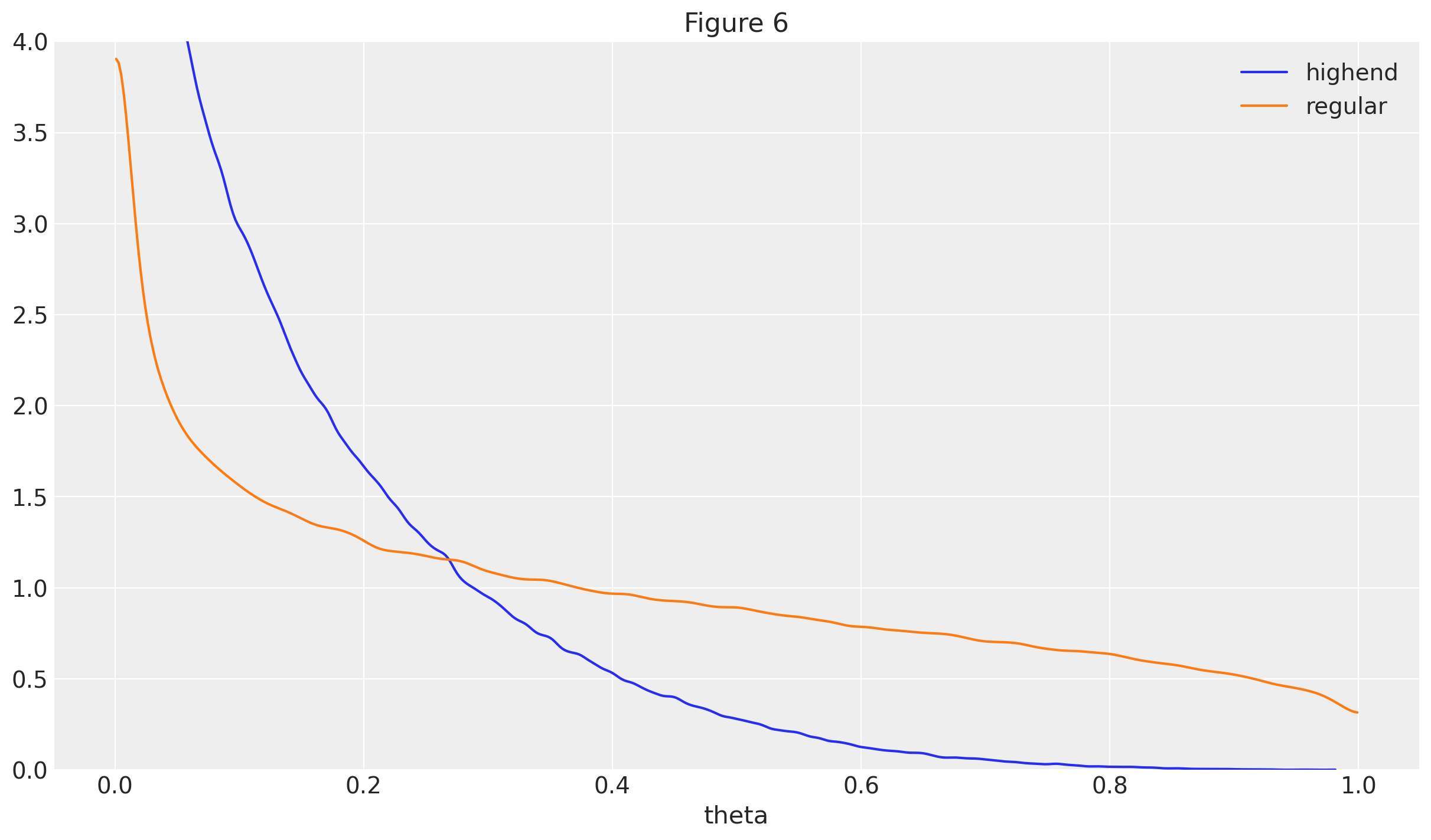
Recreating main results and figures from the paper

Figure 6 from the paper shows the group distribution of theta churn rates.

The inferred distributions are relatively wide in both groups, which follows directly from the fact that both alpha and beta were inferred to be < 10.

It is still clear that the distribution of theta for the highend users has much more mass near lower values, suggesting highend users have lower attrition rates on average, when compared with regular users.

new_highend_theta = highend_users.distribution_new_customer_theta(n=100)
new_regular_theta = regular_users.distribution_new_customer_theta(n=100);

Sampling: [theta]

100.00% [4000/4000 00:00<00:00]

Sampling: [theta]

100.00% [4000/4000 00:00<00:00]

ax = az.plot_dist(new_highend_theta, label="highend")
ax = az.plot_dist(new_regular_theta, label="regular", ax=ax, color="C1")
ax.set_xlabel("theta")
plt.ylim([0, 4])
ax.set_title("Figure 6");

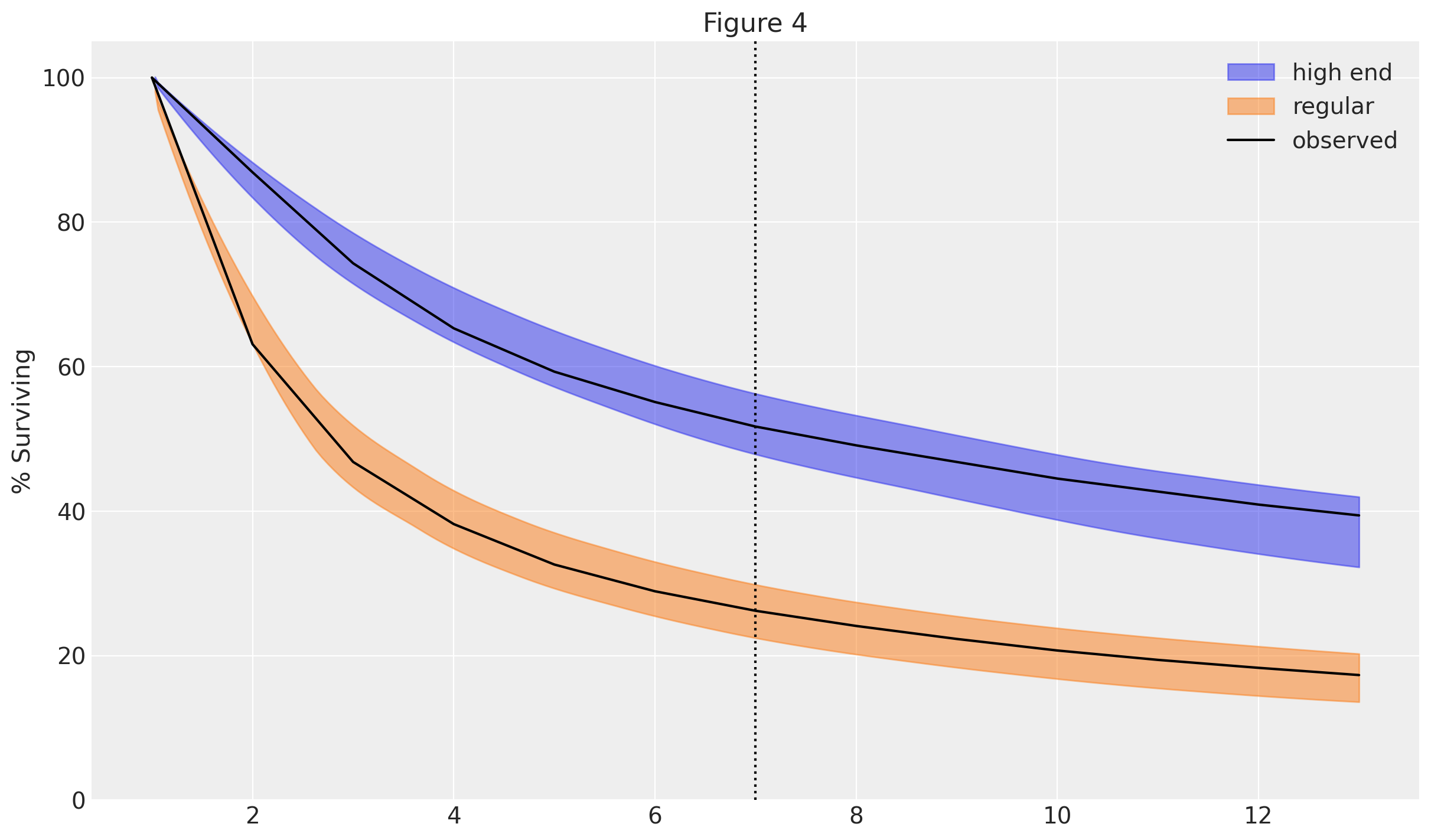
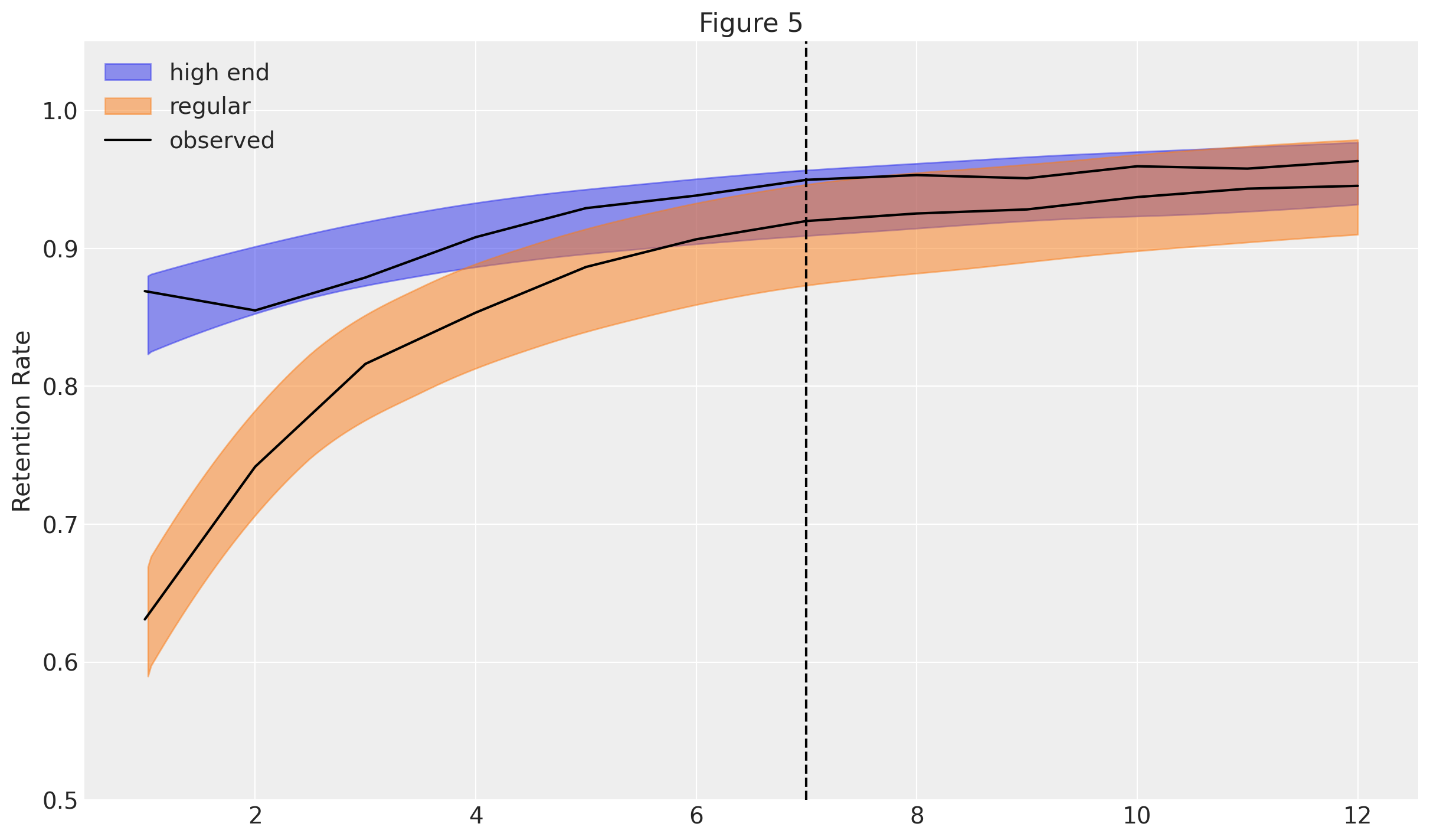
Figures 4 and 5 show the predicted average churn and retention trends for the two groups. We can see that predictions nicely match the observed data (black line), even when extrapolating into the time periods that were held-out when fitting the model.

The plots also highlight an interesting implication from the model: the retention rates are expected to increase over time, as the more precarious customers gradually drop out. This is a direct consequence of modelling individual churn rates as being fixed over time.

churn_highend = highend_users.distribution_customer_churn_time(
    customer_id=np.arange(initial_customers)
)
churn_regular = regular_users.distribution_customer_churn_time(
    customer_id=np.arange(initial_customers)
)

Sampling: [churn]

100.00% [4000/4000 00:00<00:00]

Sampling: [churn]

100.00% [4000/4000 00:00<00:00]

weeks = xr.DataArray(np.arange(1, 14), dims=["weeks"])

survival_perc_highend = 100-100*(churn_highend < weeks)
survival_perc_regular = 100-100*(churn_regular < weeks)

az.plot_hdi(weeks, survival_perc_highend.mean("customer_id"), hdi_prob=.95, color="C0")
az.plot_hdi(weeks, survival_perc_regular.mean("customer_id"), hdi_prob=.95, color="C1")

plt.plot(weeks, df["highend"], color="k", label="observed")
plt.plot(weeks, df["regular"], color="k")

plt.axvspan(None, None, color="C0", alpha=0.7, label="high end")
plt.axvspan(None, None, color="C1", alpha=0.7, label="regular")

plt.axvline(7, ls=':', color="k")
plt.ylim([0, 105])
plt.ylabel("% Surviving")
plt.legend()
plt.title("Figure 4");

retention_rate_highend = (
    survival_perc_highend.isel(weeks=slice(1, None, None))
    / survival_perc_highend.isel(weeks=slice(None, -1, None))
)
retention_rate_regular = (
    survival_perc_regular.isel(weeks=slice(1, None, None))
    / survival_perc_regular.isel(weeks=slice(None, -1, None))
)

retention_rate_highend_obs = df["highend"][1:].values / df["highend"][:-1].values
retention_rate_regular_obs = df["regular"][1:].values / df["regular"][:-1].values

weeks_ = weeks[:-1]

az.plot_hdi(weeks_, retention_rate_highend.mean("customer_id"), hdi_prob=.95, color="C0")
az.plot_hdi(weeks_, retention_rate_regular.mean("customer_id"), hdi_prob=.95, color="C1")

plt.plot(weeks_, retention_rate_highend_obs, color="k", label="observed")
plt.plot(weeks_, retention_rate_regular_obs, color="k")

plt.axvspan(None, None, color="C0", alpha=0.7, label="high end")
plt.axvspan(None, None, color="C1", alpha=0.7, label="regular")

plt.axvline(7, ls='--', color="k")
plt.ylim([0.5, 1.05])
plt.ylabel("Retention Rate")
plt.legend()
plt.title("Figure 5");