tanh_saturation_baselined#
- pymc_marketing.mmm.transformers.tanh_saturation_baselined(x, x0, gain=0.5, r=0.5)[source]#
Baselined Tanh Saturation.
This parameterization that is easier than
tanh_saturation()to use for industry applications where domain knowledge is an essence.In a nutshell, it is an alternative parameterization of the reach function is given by:
\[\begin{split}\begin{align} c_0 &= \frac{r}{g \cdot \arctan(r)} \\ \beta &= \frac{g \cdot x_0}{r} \\ \operatorname{saturation}(x, \beta, c_0) &= \beta \cdot \tanh \left( \frac{x}{c_0 \cdot \beta} \right) \end{align}\end{split}\]where:
\(x_0\) is the “reference point”. This is a point chosen by the user (not given a prior) where they expect most of their data to lie. For example, if you’re spending between 50 and 150 dollars on a particular channel, you might choose \(x_0 = 100\). Suggested value is median channel spend:
np.median(spend).\(g\) is the “gain”, which is the value of the CAC (\(c_0\)) at the reference point. You have to set a prior on what you think the CAC is when you spend \(x_0 = 100\). Imagine you have four advertising channels, and you acquired 1000 new users. If each channel performed equally well, and advertising drove all sales, you might expect that you gained 250 users from each channel. Here, your “gain” would be \(250 / 100 = 2.5\). Suggested prior is
pm.Exponential\(r\), the overspend fraction is telling you where the reference point is.
\(0\) - we can increase our budget by a lot to reach the saturated region, the diminishing returns are not visible yet.
\(1\) - the reference point is already in the saturation region and additional dollar spend will not lead to any new users.
\(0.8\), you can still increase acquired users by \(50\%\) as much you get in the reference point by increasing the budget. \(x_0\) effect is 20% away from saturation point
Suggested prior is
pm.Beta
Note
The reference point \(x_0\) has to be set within the range of the actual spends. As in, you buy ads three times and spend \(5\), \(6\) and \(7\) dollars, \(x_0\) has to be set within \([5, 7]\), so not \(4\) not \(8\). Otherwise the posterior of r and gain becomes a skinny diagonal line. It could be very relevant if there is very little spend observations for a particular channel.
The original reach or saturation function used in an MMM is formulated as
\[\operatorname{saturation}(x, \beta, c_0) = \beta \cdot \tanh \left( \frac{x}{c_0 \cdot \beta} \right)\]where:
\(\beta\) is the saturation, or the limit of the total number of new users obtained when an infinite number of dollars are spent on that channel.
\(c_0\) is the cost per acquisition (CAC0), so the initial cost per new user.
\(\frac{1}{c_0}\) is the inverse of the CAC0, so it’s the number of new users we might expect after spending our first dollar.
(
Source code,png,hires.png,pdf)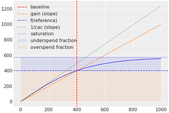
- Parameters:
- Returns:
tensorTransformed tensor.
References
Developed by Max Kochurov and Aziz Al-Maeeni doing innovative work in PyMC Labs.
Examples
import pymc as pm
import numpy as np

x_in = np.exp(3+np.random.randn(100))
true_cac = 1
true_saturation = 100
y_out = abs(np.random.normal(tanh_saturation(x_in, true_saturation, true_cac).eval(), 0.1))

with pm.Model() as model_reparam:
    r = pm.Uniform("r")
    gain = pm.Exponential("gain", 1)
    input = pm.ConstantData("spent", x_in)
    response = pm.ConstantData("response", y_out)
    sigma = pm.HalfNormal("n")
    output = tanh_saturation_baselined(input, np.median(x_in), gain, r)
    pm.Normal("output", output, sigma, observed=response)
    trace = pm.sample()